Next: Some Consequences Up: Discussion Previous: Broken-Symmetric Phase:
First of all, it is necessary to say that, regardless of the spacetime
dimension and of the symmetry group which are chosen, the dimensionless
parameters ![]() and
and ![]() are the true free parameters of the
model. Besides the requirements of stability, there is no reason to limit
their range a priori. Limitations may arise, however, from the discussion
of physically meaningful observables, expressed as expectation values,
specially in the continuum limit. We start therefore with no more than the
stability conditions that
are the true free parameters of the
model. Besides the requirements of stability, there is no reason to limit
their range a priori. Limitations may arise, however, from the discussion
of physically meaningful observables, expressed as expectation values,
specially in the continuum limit. We start therefore with no more than the
stability conditions that ![]() , and that
, and that ![]() if
if
![]() , as the limitations for
, as the limitations for ![]() and
and ![]() .
.
In the continuum limit, when we make ![]() and
and ![]() , most
dimensionless renormalized quantities we calculated here go to zero. In
order to recover the physically meaningful results in the limit, before we
take the limit we must rewrite these dimensionless quantities in terms of
the corresponding dimensionfull quantities, using the scalings listed in
Section 2, Equation (1). Since in the continuum
limit
, most
dimensionless renormalized quantities we calculated here go to zero. In
order to recover the physically meaningful results in the limit, before we
take the limit we must rewrite these dimensionless quantities in terms of
the corresponding dimensionfull quantities, using the scalings listed in
Section 2, Equation (1). Since in the continuum
limit ![]() and
and
![]() become identical, in all cases where
this is possible we will write the formulas in terms of
become identical, in all cases where
this is possible we will write the formulas in terms of ![]() only,
producing in this way equations which are equivalent to the original ones
for the purposes of that limit.
only,
producing in this way equations which are equivalent to the original ones
for the purposes of that limit.
Starting with the expectation value of the field, in the case in which
there is no external source ![]() , in which case the limit must be taken
within the broken-symmetric phase of the model if we are to have the
possibility of a non-zero result, from Equation (7) we have
, in which case the limit must be taken
within the broken-symmetric phase of the model if we are to have the
possibility of a non-zero result, from Equation (7) we have
![\begin{eqnarray*}
\left\langle\phi_{\mathfrak{N}}(x_{\mu})\right\rangle
& = &
...
...rak{N}+2)\sigma_{0}^{2}\right]}}
{\sqrt{\lambda}\,a^{(d-2)/2}}.
\end{eqnarray*}](img182.png)
Since for ![]() the denominator goes to zero in the continuum limit,
if the field
the denominator goes to zero in the continuum limit,
if the field
![]() is to have a finite expectation value,
then it is necessary that
is to have a finite expectation value,
then it is necessary that ![]() approach zero in the limit, which
forcefully takes us to points over the critical line, which is
characterized by
approach zero in the limit, which
forcefully takes us to points over the critical line, which is
characterized by ![]() and by the equation that states that the
quantity within the square root above is zero.
and by the equation that states that the
quantity within the square root above is zero.
Since the critical line starts at the Gaussian point and extends to the
quadrant where ![]() and
and ![]() , it follows that all
possible continuum limits originating from the broken-symmetric phase must
go to points in the parameter plane where
, it follows that all
possible continuum limits originating from the broken-symmetric phase must
go to points in the parameter plane where ![]() , the case
, the case
![]() being the Gaussian point and corresponding to the Gaussian
sector of the model. In
being the Gaussian point and corresponding to the Gaussian
sector of the model. In ![]() , in particular, all possible
non-trivial continuum limits necessarily correspond to strictly negative
values of
, in particular, all possible
non-trivial continuum limits necessarily correspond to strictly negative
values of ![]() . A particular sequence of values of
. A particular sequence of values of
![]() approaching the critical line defines both a path in the parameter space
of the model and a rate of progress along that path, leading to that
particular continuum limit, and is called a continuum limit flow. A
continuum limit is completely characterized by its flow, and is not
characterized completely just by a point
approaching the critical line defines both a path in the parameter space
of the model and a rate of progress along that path, leading to that
particular continuum limit, and is called a continuum limit flow. A
continuum limit is completely characterized by its flow, and is not
characterized completely just by a point
![]() in the
parameter plane.
in the
parameter plane.
Going back to the case in which we have an external source present, we may now rewrite Equation (9) in terms of the renormalized dimensionfull quantities, thus obtaining
In the case ![]() we see that, if
we see that, if ![]() is not zero, then the first
term dominates over the others, and therefore we conclude simply that
is not zero, then the first
term dominates over the others, and therefore we conclude simply that
![]() . It follows that in this case there is no spontaneous
symmetry breaking and no effect of the external source over
. It follows that in this case there is no spontaneous
symmetry breaking and no effect of the external source over ![]() in the
continuum limit. If we wish to have any interesting structure in the model
in this case, we are forced to make
in the
continuum limit. If we wish to have any interesting structure in the model
in this case, we are forced to make ![]() in the limit. If we do
that at the appropriate rate, there may be interesting continuum limits
sitting right over the Gaussian point. In the case
in the limit. If we do
that at the appropriate rate, there may be interesting continuum limits
sitting right over the Gaussian point. In the case ![]() , on the other
hand, we see that the first term vanishes, and we are left with
, on the other
hand, we see that the first term vanishes, and we are left with
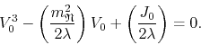
![]() , which is characteristic of a free, or trivial
theory. In the case
, which is characteristic of a free, or trivial
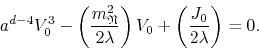
theory. In the case ![]() we get the equation
we get the equation
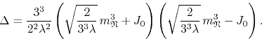
It is interesting to calculate the discriminant ![]() of this cubic
equation, which turns out to be
of this cubic
equation, which turns out to be
We can see now that the number of roots of the equation depends on the
value of ![]() in a simple way. If we have
in a simple way. If we have
then ![]() and therefore there are three distinct simple real
roots. If we have
and therefore there are three distinct simple real
roots. If we have
then ![]() and the three roots merge into one triple real root.
Finally, if
and the three roots merge into one triple real root.
Finally, if
then ![]() and there is a single real root, the other two having
non-zero imaginary parts. This supports the idea that as
and there is a single real root, the other two having
non-zero imaginary parts. This supports the idea that as ![]() increases
along positive values, the left well of the potential becomes shallower
and eventually there is no possibility for the local distribution of the
field
increases
along positive values, the left well of the potential becomes shallower
and eventually there is no possibility for the local distribution of the
field
![]() to fit within it, even to form a meta-stable state.
One of the roots relates to the third extremum of the potential, the local
maximum between the two minima. It is clear that, when there is more than
one solution to the equation, only the largest solution corresponds to a
stable state and is therefore relevant in the context of the symmetry
breaking driven by a positive
to fit within it, even to form a meta-stable state.
One of the roots relates to the third extremum of the potential, the local
maximum between the two minima. It is clear that, when there is more than
one solution to the equation, only the largest solution corresponds to a
stable state and is therefore relevant in the context of the symmetry
breaking driven by a positive ![]() .
.
The same analysis regarding critical behavior and the critical line is
valid for the renormalized masses. Considering first the limits from the
symmetric phase, with no external source ![]() , we have
, we have
![]() with
with
![]() , and therefore
using Equation (10) we have
, and therefore
using Equation (10) we have
We can see that, regardless of how we take the limit, we will necessarily
have
![]() in this case. Observe that the numerator on the
right-hand side is the quantity which, according to the equation of the
critical line, is zero over that line, and hence approaches zero when
in this case. Observe that the numerator on the
right-hand side is the quantity which, according to the equation of the
critical line, is zero over that line, and hence approaches zero when
![]() tends to a point on the critical line. Once more we see
that, if we are to have a finite value for
tends to a point on the critical line. Once more we see
that, if we are to have a finite value for ![]() , we must approach the
critical line on the continuum limit, in such a way that the quantity
, we must approach the
critical line on the continuum limit, in such a way that the quantity
![]() approaches zero as
approaches zero as ![]() or
faster. If the approach is such that the quantity in the numerator behaves
exactly as
or
faster. If the approach is such that the quantity in the numerator behaves
exactly as ![]() , then we have a finite and non-zero value of
, then we have a finite and non-zero value of ![]() .
If the approach is faster than that, then we will have
.
If the approach is faster than that, then we will have ![]() . On the
other hand, if it is too slow, then we may end up with an infinite
. On the
other hand, if it is too slow, then we may end up with an infinite ![]() in the limit.
in the limit.
The same type of mechanism works for limits from the broken-symmetric
phase, except that in that case we will always have ![]() in the
limit, as we will now demonstrate. As we saw before in
Equation (11), we have for
in the
limit, as we will now demonstrate. As we saw before in
Equation (11), we have for ![]()
which indeed goes to zero in the limit. However, the analysis of the limit
is not so simple, due to the fact that on finite lattices ![]() appears in the right-hand side of the equation as well. If we write it
explicitly, using Equations (B.6) and (B.7) of
Appendix B, we get an equation involving
appears in the right-hand side of the equation as well. If we write it
explicitly, using Equations (B.6) and (B.7) of
Appendix B, we get an equation involving ![]() and
and
![]() ,
,
![\begin{eqnarray*}
\alpha_{0}
& = &
2\lambda\,
\frac{1}{N^{d}}
\sum_{k_{\mu}...
...right]
\left[\rho^{2}(k_{\mu})+\alpha_{\mathfrak{N}}\right]
}.
\end{eqnarray*}](img206.png)
Now, if
![]() , which implies that
, which implies that
![]() ,
then the right-hand side is zero, and therefore so is
,
then the right-hand side is zero, and therefore so is ![]() . This
in turn implies that
. This
in turn implies that ![]() , as expected. This is in fact one
possibility, we may indeed have both
, as expected. This is in fact one
possibility, we may indeed have both ![]() and
and
![]() zero in the
limit. If, on the other hand, we have
zero in the
limit. If, on the other hand, we have
![]() , then
we may write the equation as
, then
we may write the equation as
![\begin{displaymath}
\frac{m_{0}^{2}}{m_{\mathfrak{N}}^{2}-m_{0}^{2}}
=
2\lamb...
...ght]
\left[\rho^{2}(k_{\mu})+\alpha_{\mathfrak{N}}\right]
},
\end{displaymath}](img210.png)
where we wrote the left-hand side in terms of dimensionfull quantities.
Obviously, because both ![]() and the sum are necessarily positive
quantities, it is impossible to have
and the sum are necessarily positive
quantities, it is impossible to have
![]() . Here we see that, if
we have both
. Here we see that, if
we have both ![]() and
and
![]() different from zero in the limit,
then the left-hand side has a non-zero limit and therefore the normalized
sum on the right-hand side must be non-zero in the limit.
different from zero in the limit,
then the left-hand side has a non-zero limit and therefore the normalized
sum on the right-hand side must be non-zero in the limit.
However, one can check numerically that, for ![]() and in the type of
continuum limit that we consider here, the normalized sum does indeed go
to zero in the limit. This implies that in these dimensions, which include
and in the type of
continuum limit that we consider here, the normalized sum does indeed go
to zero in the limit. This implies that in these dimensions, which include
![]() , we cannot have both
, we cannot have both ![]() and
and
![]() different from zero in
the limit. Since
different from zero in
the limit. Since
![]() , this implies that we must always have
, this implies that we must always have
![]() in the limit. What we have here, as one should expect, are the
Goldstone bosons brought about by the process of spontaneous symmetry
breaking.
in the limit. What we have here, as one should expect, are the
Goldstone bosons brought about by the process of spontaneous symmetry
breaking.
For the longitudinal mass parameter
![]() we have, using
Equation (13),
we have, using
Equation (13),
![\begin{eqnarray*}
\alpha_{\mathfrak{N}}
& = &
-2
\left[\alpha+\lambda(\mathf...
...left[\alpha+\lambda(\mathfrak{N}+2)\sigma_{0}^{2}\right]}}
{a},
\end{eqnarray*}](img214.png)
so that exactly the same argument that was used for ![]() in the
symmetric phase applies. We see therefore that the need to approach the
critical line when one takes continuum limits in this model is a rather
general characteristic of the model. This makes the critical line the
locus of all physically possible continuum limits of the model.
This means that making
in the
symmetric phase applies. We see therefore that the need to approach the
critical line when one takes continuum limits in this model is a rather
general characteristic of the model. This makes the critical line the
locus of all physically possible continuum limits of the model.
This means that making ![]() is not a choice that we have, since it
is forced upon us by the need to obtain physically meaningful
continuum limits.
is not a choice that we have, since it
is forced upon us by the need to obtain physically meaningful
continuum limits.
Let us now discuss the continuum limits of the transversal renormalized mass in the presence of an external source. We have the result in Equation (5), valid in either phase,
Observe that this equation implies that it is still necessary to approach
the critical line in the continuum limit, and in the same ways as before.
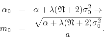
In the symmetric phase, if ![]() is the corresponding result in
the absence of external sources, which corresponds to
is the corresponding result in
the absence of external sources, which corresponds to ![]() , we may
write
, we may
write
Rewriting all quantities in terms of the corresponding dimensionfull ones we have
We see that for ![]() we are forced to make
we are forced to make ![]() in the limit.
In the case
in the limit.
In the case ![]() no additional constraints on
no additional constraints on ![]() arise, and we get
the relation
arise, and we get
the relation
describing indirectly how ![]() increases with
increases with ![]() through
the variation of
through
the variation of ![]() . In the case
. In the case ![]() the term containing
the term containing ![]() vanishes in the limit, and we get simply that
vanishes in the limit, and we get simply that
![]() ,
meaning that in this case
,
meaning that in this case ![]() does not really depend on
does not really depend on ![]() in the continuum limit.
in the continuum limit.
In the broken-symmetric phase we may start with Equation (12)
for the transversal mass parameter. If we recall that we have already
shown that in this phase we must have ![]() in the limit, we may
make
in the limit, we may
make
![]() in this formula and thus obtain
in this formula and thus obtain
In terms of dimensionfull quantities we have therefore
which gives us back ![]() in the absence of external sources. Not
much changes in the discussion of the various possible dimensions. We may
restrict our comments to the case
in the absence of external sources. Not
much changes in the discussion of the various possible dimensions. We may
restrict our comments to the case ![]() , in which we get a fairly simple
relation giving
, in which we get a fairly simple
relation giving ![]() in the presence of the external source,
in the presence of the external source,
The same analysis can be made for the longitudinal mass in the presence of an external source. In this case we have the result in Equation (6), valid in either phase,
The necessity to approach the critical line remains in force here. In the
symmetric phase, if
![]() is the corresponding result in the
absence of external sources, which corresponds to
is the corresponding result in the
absence of external sources, which corresponds to ![]() , we may write
, we may write
Rewriting all quantities in terms of the corresponding dimensionfull ones we have
Once more we see that for ![]() we are forced to make
we are forced to make ![]() in
the limit. In the case
in
the limit. In the case ![]() we get simply the relation
we get simply the relation
describing indirectly how
![]() increases with
increases with ![]() through
the variation of
through
the variation of ![]() . In the case
. In the case ![]() the term containing
the term containing ![]() vanishes in the limit, and we get simply that
vanishes in the limit, and we get simply that
![]() ,
meaning that in this case
,
meaning that in this case
![]() also does not depend on
also does not depend on ![]() in the continuum limit.
in the continuum limit.
In the broken-symmetric phase we may start with Equation (14) for the longitudinal mass parameter
where
![]() is the value of the parameter in the
absence of external sources. In terms of dimensionfull quantities we have
therefore
is the value of the parameter in the
absence of external sources. In terms of dimensionfull quantities we have
therefore
Once again not much changes in the discussion of the various possible
dimensions. In the case ![]() we get
we get
It is interesting to note that, both for the transversal and longitudinal
masses, the dependence of the renormalized masses on the external source
![]() seems to be a peculiar feature of the case
seems to be a peculiar feature of the case ![]() , which is absent
for
, which is absent
for ![]() .
.