Next: Calculations Up: Gaussian-Perturbative Calculations with a Previous: Introduction
Let us start by giving the definition of the model, in the classical and
quantum domains, and then quickly reviewing the Gaussian-Perturbative
approximation. Consider then the Euclidean quantum field theories of an
![]() -symmetric set of scalar fields
-symmetric set of scalar fields
![]() defined
within a periodical cubic box of side
defined
within a periodical cubic box of side ![]() in
in ![]() dimensions by the
classical action
dimensions by the
classical action
![\begin{eqnarray*}
S\!\left[\raisebox{-0.3ex}{$\vec{\phi}$}\right]
& = &
\oint...
...mu})\right]^{2}
-
J_{0}\phi_{\mathfrak{N}}(x_{\mu})
\right\},
\end{eqnarray*}](img18.png)
where ![]() . This is the usual form of the
. This is the usual form of the
![]() -symmetric
-symmetric
![]() model in the classical continuum, with an external
source
model in the classical continuum, with an external
source ![]() , which by assumption is a constant. The vector notation
, which by assumption is a constant. The vector notation
![]() is shorthand for
is shorthand for
and the dot-product notation represents the scalar product of vectors in
the internal
![]() space, that is a sum over
space, that is a sum over
![]() ,
,
![\begin{displaymath}
\vec{\phi}(x_{\mu})\cdot\vec{\phi}(x_{\mu})
=
\sum_{i}^{\mathfrak{N}}
\left[\phi_{i}(x_{\mu})\right]^{2}.
\end{displaymath}](img22.png)
In this action the quantity ![]() is a homogeneous external source
associated with the
is a homogeneous external source
associated with the
![]() field component. Its
introduction breaks the
field component. Its
introduction breaks the
![]() symmetry, of course, and causes the
generation of a non-zero expectation value for the
symmetry, of course, and causes the
generation of a non-zero expectation value for the
![]() field component.
field component.
In order to use the definition of the quantum theory on a cubical lattice
of size ![]() with
with ![]() sites along each direction, with lattice spacing
sites along each direction, with lattice spacing
![]() , we consider the corresponding lattice action
, we consider the corresponding lattice action
![\begin{eqnarray*}
S_{N}[\vec{\varphi}]
& = &
\sum_{n_{\mu}}^{N^{d}}
\left\{
...
...)\right]^{2}
-
j_{0}\varphi_{\mathfrak{N}}(n_{\mu})
\right\},
\end{eqnarray*}](img26.png)
where all quantities are now dimensionless, defined by the appropriate scalings,
In order for the model to be stable we must have ![]() and, in
addition to this, if
and, in
addition to this, if ![]() then we must also have
then we must also have ![]() . Up
to this point there are no further constraints on the real parameters
. Up
to this point there are no further constraints on the real parameters
![]() and
and ![]() .
.
When possible, the summations are notated, in the subscript, by the
variable which is being summed over, and, in the superscript, by the
number of terms in the sum. The integer coordinates ![]() are taken to
vary as symmetrically as possible around the origin
are taken to
vary as symmetrically as possible around the origin
![]() ,
that is we have
,
that is we have
![]() with
certain values of
with
certain values of ![]() and
and ![]() that depend on the
parity of
that depend on the
parity of ![]() ,
,
for odd ![]() , and
, and
for even ![]() , in either case for all values of
, in either case for all values of
![]() .
.
In this paper we will perform the calculations of the critical line and of
the renormalized masses in a situation in which we have, in terms of the
dimensionfull field
![]() , for
, for
![]() ,
,
and, for
![]() ,
,
where ![]() is a constant with the physical dimensions of the field
is a constant with the physical dimensions of the field
![]() . In terms of the dimensionless field
. In terms of the dimensionless field
![]() we have for the only non-trivial condition
we have for the only non-trivial condition
where the dimensionless constant is given by
![]() .
.
We will consider continuum limits in which we have both ![]() and
and
![]() . In order to do this we will choose to make
. In order to do this we will choose to make ![]() increase as
increase as
![]() and
and ![]() decrease as
decrease as ![]() , so that we still have
, so that we still have
![]() . The calculations on finite lattices will be performed with
periodical boundary conditions, with the understanding that at the end of
the day such a limit is to be taken.
. The calculations on finite lattices will be performed with
periodical boundary conditions, with the understanding that at the end of
the day such a limit is to be taken.
Observe that we are specifying the value of the expectation value ![]() of
of
![]() rather than the value of the corresponding
external source
rather than the value of the corresponding
external source ![]() . What we are doing here is to assume that there is
some external source present such that we have the expectation value
specified. It follows that one of the expected results of our calculations
is the determination, at least implicitly, of the form of the external
source in terms of
. What we are doing here is to assume that there is
some external source present such that we have the expectation value
specified. It follows that one of the expected results of our calculations
is the determination, at least implicitly, of the form of the external
source in terms of ![]() .
.
Our first calculational task in preparation for the Gaussian-Perturbative
calculations is to rewrite the action in terms of a shifted field, which
has a null expectation value. We thus define a new field variable
![]() such that
such that
so that we have
![]() for
all
for
all ![]() , with
, with
![]() . We must now determine the form of
the action in terms of
. We must now determine the form of
the action in terms of
![]() . If we write each term of
the action in terms of the shifted field we get
. If we write each term of
the action in terms of the shifted field we get
![\begin{eqnarray*}
S_{N}[\vec{\varphi}']
& = &
\sum_{n_{\mu}}^{N^{d}}
\left\{...
... j_{0}\varphi_{\mathfrak{N}}'(n_{\mu})
-
j_{0}v_{0}
\right\}.
\end{eqnarray*}](img67.png)
We will now eliminate all field-independent terms, since they correspond to constant factors that cancel off in the ratios of functional integrals which give the expectation values of the observables. Doing this we get the equivalent action
![\begin{eqnarray*}
S_{N}[\vec{\varphi}']
& = &
\sum_{n_{\mu}}^{N^{d}}
\left\{...
...phi}'(n_{\mu})\cdot\vec{\varphi}'(n_{\mu})\right]^{2}
\right\},
\end{eqnarray*}](img68.png)
where except for the kinetic part the terms have been ordered by increasing powers of the field.
The last task we have to perform, in preparation for the
Gaussian-Perturbative calculations, is the separation of the action in two
parts. Since the symmetry is broken by the introduction of the external
sources, besides the fact that depending on the values of the parameters
![]() and
and ![]() it might be spontaneously broken as well, this
separation involves two new mass parameters,
it might be spontaneously broken as well, this
separation involves two new mass parameters, ![]() for
for
![]() , and
, and
![]() for
for
![]() . Note that an
. Note that an
![]() symmetry subgroup is left over after the
symmetry subgroup is left over after the
![]() symmetry breakdown. We
therefore adopt for the Gaussian part of the action
symmetry breakdown. We
therefore adopt for the Gaussian part of the action
where there are no constraints on the parameters introduced other than
![]() and
and
![]() . Note that, despite the way in
which this is written, we do in fact have here just an
. Note that, despite the way in
which this is written, we do in fact have here just an ![]() mass
term for each field component
mass
term for each field component
![]() , for
, for
![]() , and an
, and an
![]() mass term for the field
component
mass term for the field
component
![]() . It follows that the non-Gaussian part
of the action is
. It follows that the non-Gaussian part
of the action is
which has its terms now written strictly in the order of increasing powers of the field.
Let us end this section by recalling the calculational techniques that
will be involved. Given an arbitrary observable
![]() its
expectation value is defined by
its
expectation value is defined by
![\begin{displaymath}
\left\langle{\mathbf O}[\vec{\varphi}']\right\rangle
=
\f...
...i]\,
e^{-S_{0}[\vec{\varphi}']-\xi S_{V}[\vec{\varphi}']}
},
\end{displaymath}](img85.png)
which is a function of ![]() , where
, where
![]() denotes the flat
measure and hence integrals from
denotes the flat
measure and hence integrals from ![]() to
to ![]() over all the field
components at all sites. The expectation values of the model are obtained
for
over all the field
components at all sites. The expectation values of the model are obtained
for ![]() , and the corresponding expectation values in the Gaussian
measure of
, and the corresponding expectation values in the Gaussian
measure of
![]() are those obtained for
are those obtained for ![]() . The
Gaussian-Perturbative approximation consists of the expansion of the
right-hand side in powers of
. The
Gaussian-Perturbative approximation consists of the expansion of the
right-hand side in powers of ![]() to some finite order, around the point
to some finite order, around the point
![]() , and the application of the resulting expression at
, and the application of the resulting expression at ![]() . The
first-order Gaussian-Perturbative approximation of the expectation value
of the observable
. The
first-order Gaussian-Perturbative approximation of the expectation value
of the observable
![]() is given by
is given by
where the subscript ![]() indicates the expectation values in the measure of
indicates the expectation values in the measure of
![]() . These expectation values are most easily
calculated in momentum space, where they involve only uncoupled Gaussian
integrals. Therefore, let us also recall here the transformations to and
from the momentum space representation of the model. We have for the field
and its Fourier transform
. These expectation values are most easily
calculated in momentum space, where they involve only uncoupled Gaussian
integrals. Therefore, let us also recall here the transformations to and
from the momentum space representation of the model. We have for the field
and its Fourier transform
![]()
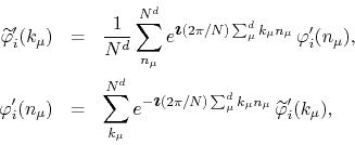
where the sums over ![]() are taken in as symmetric a way as possible
around
are taken in as symmetric a way as possible
around
![]() , just as we did for
, just as we did for ![]() . In other words, we
have
. In other words, we
have
![]() with the same
values of
with the same
values of ![]() and
and ![]() , depending on the parity of
, depending on the parity of ![]() ,
that were used for
,
that were used for ![]() and
and ![]() ,
,
for odd ![]() , and
, and
for even ![]() , in either case for all values of
, in either case for all values of
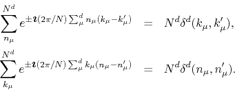
![]() . The
orthogonality and completeness relations of the Fourier base are given by
. The
orthogonality and completeness relations of the Fourier base are given by
A typical Gaussian expectation value in momentum space, and possibly the most fundamental one, is given for a generic field component by
where ![]() is either
is either ![]() or
or
![]() , depending on
the field component involved, and where
, depending on
the field component involved, and where
![]() are the
eigenvalues of the discrete Laplacian on the lattice, which are given by
are the
eigenvalues of the discrete Laplacian on the lattice, which are given by
This and several other expectation values, Gaussian integration formulas and lattice sums can be found in Appendix B.
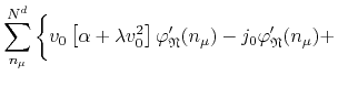
![$\displaystyle \sum_{n_{\mu}}^{N^{d}}
\left\{
\rule{0em}{4ex}
\frac{1}{2}
\sum_{...
...{\varphi}'(n_{\mu})
\cdot
\Delta_{\nu}\vec{\varphi}'(n_{\mu})
\right]
+
\right.$](img75.png)
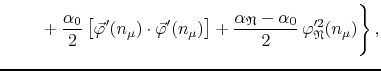
![$\displaystyle \hspace{2.0em}
\left.
\rule{0em}{3ex}
+
\lambda
v_{0}
\left[\vec{...
...
\left[\vec{\varphi}'(n_{\mu})\cdot\vec{\varphi}'(n_{\mu})\right]^{2}
\right\},$](img83.png)