The Transversal Propagator

We will now calculate the expectation value of the observable

$${\mathbf O}[\vec{\varphi}'] = \varphi_{i}'(n_{\mu}') \varphi_{i}'(n_{\mu}''),$$

which has the same form for all components of the field except $i=\mathfrak{N}$. We call this the transversal propagator because it belongs to the field components which are orthogonal to the direction of the external source in the internal $SO(\mathfrak{N})$ space. In this section we will assume that $i\neq\mathfrak{N}$, in fact we will make $i=1$. The observable will be taken at two arbitrary points $n_{\mu}'$ and $n_{\mu}''$. The first-order Gaussian-Perturbative approximation for this observable gives

$$\begin{eqnarray*} \left\langle \varphi_{1}'(n_{\mu}') \varphi_{1}'(n_{\mu}'')... ...left\langle S_{V}[\vec{\varphi}'] \right\rangle_{0} \right\}, \end{eqnarray*}$$

where $g_{0}(n_{\mu}'-n_{\mu}'')$ is the two-point function with mass parameter $\alpha_{0}$. We must calculate the two expectation values which appear in this formula. The calculation of the first one is done in Appendix A, given in Equation (A.5), and results in

$$\begin{eqnarray*} \left\langle S_{V}[\vec{\varphi}'] \right\rangle_{0} & = &... ...2} + \frac{3\lambda}{4}\, \sigma_{\mathfrak{N}}^{4} \right]. \end{eqnarray*}$$

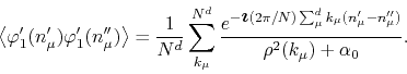
The second expectation value is also calculated in Appendix A, given in Equation (A.6), and the result is

$$\begin{eqnarray*} \lefteqn { \left\langle \varphi_{1}'(n_{\mu}') \varphi_{1... ...{\mu}'-n_{\mu}'')} } { [\rho^{2}(k_{\mu})+\alpha_{0}]^{2} }. \end{eqnarray*}$$

The factor in front of $g_{0}(n_{\mu}'-n_{\mu}'')$ can now be verified to be exactly equal to $\left\langle S_{V}[\vec{\varphi}']\right\rangle_{0}$, and therefore this whole part cancels off from our observable. We may now write for the difference of expectation values that appears in it,

$$\begin{eqnarray*} \lefteqn { \left\langle \varphi_{1}'(n_{\mu}') \varphi_{1... ...{\mu}'-n_{\mu}'')} } { [\rho^{2}(k_{\mu})+\alpha_{0}]^{2} }. \end{eqnarray*}$$

Finally, we can write the complete result,

$$\begin{eqnarray*} \lefteqn { \left\langle \varphi_{1}'(n_{\mu}') \varphi_{1... ...athfrak{N}}^{2} } { \rho^{2}(k_{\mu})+\alpha_{0} } \right], \end{eqnarray*}$$

where we wrote $g_{0}(n_{\mu}'-n_{\mu}'')$ in terms of its Fourier transform.

In principle we could have used any positive value of $\alpha_{0}$ for this calculation, but now a particular choice comes to our attention. We see from the structure of this propagator that we can make $\alpha_{0}$ equal to the transversal renormalized mass parameter by choosing it so that the numerator of the second fraction vanishes. In this way we get a very simple propagator, with a simple pole in the complex $\rho^{2}$ plane, in which the parameter $\alpha_{0}$ appears now in the role of the renormalized mass parameter,

$$\left\langle \varphi_{1}'(n_{\mu}') \varphi_{1}'(n_{\mu}'... ...}(n_{\mu}'-n_{\mu}'')} } { \rho^{2}(k_{\mu})+\alpha_{0} }.$$

Observe that to this order the propagator is, in fact, the propagator of the free theory. This is a self-consistent way to choose the parameter $\alpha_{0}$, and is equivalent to the determination of the transversal renormalized mass. This choice is equivalent to requiring that the mass parameter of the Gaussian measure being used for the approximation of the expectation values be the same as the renormalized mass parameter of the original quantum model. It gives the result

$$\alpha_{0} = \lambda v_{0}^{2} + \alpha + \lambda \... ...{N}+1) \sigma_{0}^{2} + \sigma_{\mathfrak{N}}^{2} \right].$$ (C.5)

This result for $\alpha_{0}=a^{2}m_{0}^{2}$ is valid for a constant but possibly non-zero external source, in both phases of the model, where $m_{0}$ is the mass associated to the $\mathfrak{N}-1$ field components $\varphi_{i}'(n_{\mu})$, for $i\neq\mathfrak{N}$.