Next: The Convergence Condition Up: Complex Analysis of Real Previous: An Infinite Collection of
We will now derive certain expressions for the partial sums and for the
corresponding remainders of the Fourier series. In order to do this, let
![]() be a zero-average integrable real function defined on
be a zero-average integrable real function defined on
![]() and let the real numbers
and let the real numbers ![]() ,
, ![]() and
and
![]() , for
, for
![]() , be its Fourier
coefficients. We then define the complex coefficients
, be its Fourier
coefficients. We then define the complex coefficients ![]() and
and
![]() shown in Equation (5), and thus construct the
corresponding proper inner analytic function
shown in Equation (5), and thus construct the
corresponding proper inner analytic function ![]() within the open unit
disk, using the power series
within the open unit
disk, using the power series ![]() given in Equation (6),
which, as was shown in [#!CAoRFI!#], always converges for
given in Equation (6),
which, as was shown in [#!CAoRFI!#], always converges for
![]() . Considering that
. Considering that ![]() , the partial sums of the first
, the partial sums of the first
![]() terms of this series are given by
terms of this series are given by
where
![]() , a complex sequence for each value of
, a complex sequence for each value of
![]() which, for
which, for ![]() , we already know to converge to
, we already know to converge to ![]() in the
in the
![]() limit. Note however that, since
limit. Note however that, since ![]() is a polynomial of
order
is a polynomial of
order ![]() and therefore an analytic function over the whole complex plane,
this expression itself can be consistently considered for all finite
and therefore an analytic function over the whole complex plane,
this expression itself can be consistently considered for all finite ![]() and all
and all ![]() , and in particular for
, and in particular for ![]() on the unit circle, where
on the unit circle, where ![]() .
One can also define the corresponding remainders of the complex power
series, in the usual way, as
.
One can also define the corresponding remainders of the complex power
series, in the usual way, as
We will now prove the following theorem.
![$\displaystyle \frac{1}{2\pi}\,
\int_{-\pi}^{\pi}d\theta_{1}\,
\frac
{
\sin\!\le...
...0em}{2ex}(N+1/2)\Delta\theta\right]
}
{
\sin(\Delta\theta/2)
}\,
f(\theta_{1}),$](img209.png) |
|||
![$\displaystyle \frac{1}{2\pi}\,
\mbox{\rm PV}\!\!\int_{-\pi}^{\pi}d\theta_{1}\,
...
...0em}{2ex}(N+1/2)\Delta\theta\right]
}
{
\sin(\Delta\theta/2)
}\,
g(\theta_{1}),$](img211.png) |
(53) |
where
![]() and
and
![]() .
.
Note that the integral in the expression of the partial sum is the known Dirichlet integral, while the one in the expression of the reminder is similar but not identical to it.
In order to prove this theorem, let us consider the complex partial sums
![]() as given in Equation (51). In addition to this,
the complex coefficients
as given in Equation (51). In addition to this,
the complex coefficients ![]() may be written as integrals involving
may be written as integrals involving
![]() , with the use of the Cauchy integral formulas,
, with the use of the Cauchy integral formulas,
| (54) |
for
![]() , where
, where ![]() can be taken as a circle
centered at the origin, with radius
can be taken as a circle
centered at the origin, with radius ![]() . The reason why we may
include the case
. The reason why we may
include the case ![]() here is that, as was shown in [#!CAoRFI!#], as
a function of
here is that, as was shown in [#!CAoRFI!#], as
a function of ![]() the expression above for
the expression above for ![]() is not only constant
within the open unit disk, but also continuous from within at the unit
circle. In this way the coefficients
is not only constant
within the open unit disk, but also continuous from within at the unit
circle. In this way the coefficients ![]() may be written back in terms
of the inner analytic function
may be written back in terms
of the inner analytic function ![]() . If we substitute this expression
for
. If we substitute this expression
for ![]() back in the partial sums of the complex power series shown in
Equation (51) we get
back in the partial sums of the complex power series shown in
Equation (51) we get
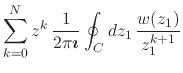 |
|||
 |
(55) |
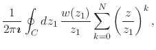
where ![]() can have any value, but where we must have
can have any value, but where we must have ![]() . The
sum is now a finite geometric progression, so that we have its value in
closed form,
. The
sum is now a finite geometric progression, so that we have its value in
closed form,
 |
|||
 |
(56) |
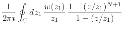
There are now two relevant cases to be considered here, the case in which
![]() and the case in which
and the case in which ![]() . In the first case,
since the explicit simple pole of the integrand at the position
. In the first case,
since the explicit simple pole of the integrand at the position ![]() lies within the integration contour, we have in the first term the Cauchy
integral formula for
lies within the integration contour, we have in the first term the Cauchy
integral formula for ![]() , and therefore we get
, and therefore we get
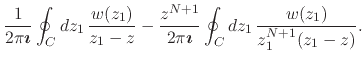
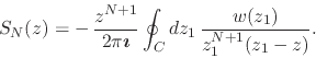
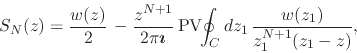
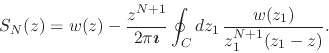
This is the equation that allows us to write an explicit expression for
the remainder of the complex power series within the open unit disk, thus
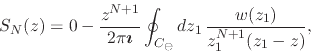
making it easier to discuss its convergence there. In the other case, in
which ![]() , the explicit simple pole of the integrand at the
position
, the explicit simple pole of the integrand at the
position ![]() lies outside of the integration contour, and therefore by the
Cauchy-Goursat theorem we just have zero in the first term, so that we get
lies outside of the integration contour, and therefore by the
Cauchy-Goursat theorem we just have zero in the first term, so that we get
 |
(58) |
This provides us, therefore, with an explicit expression for the partial
sums, but not for the remainder. The only other possible case is that in
which ![]() , in which both
, in which both ![]() and
and ![]() are over the circle
are over the circle ![]() of radius
of radius ![]() , and therefore so is the explicit simple pole of the
integrand at the position
, and therefore so is the explicit simple pole of the
integrand at the position ![]() . In this case, just as we did before
in Section 3, we may slightly deform the integration contour
. In this case, just as we did before
in Section 3, we may slightly deform the integration contour ![]() in order to have it pass on one side or the other of the simple pole of
the integrand at
in order to have it pass on one side or the other of the simple pole of
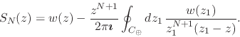
the integrand at ![]() . If we use a deformed contour
. If we use a deformed contour ![]() that excludes the pole from its interior, then we have, instead of
Equation (57),
that excludes the pole from its interior, then we have, instead of
Equation (57),
while if we use a deformed contour ![]() that includes the
pole in its interior, then we have, just as in
Equation (57),
that includes the
pole in its interior, then we have, just as in
Equation (57),
Once more, since by the Sokhotskii-Plemelj theorem [#!sokhplem!#] the
Cauchy principal value of the integral over ![]() is the arithmetic average
of these two integrals, taking the average of
Equations (59) and (60) we obtain the
expression
is the arithmetic average
of these two integrals, taking the average of
Equations (59) and (60) we obtain the
expression
 |
(61) |
where both ![]() and
and ![]() are now on the circle
are now on the circle ![]() of radius
of radius ![]() .
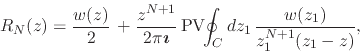
Since we have that the corresponding remainder of the series is defined as
given in Equation (52), we get a corresponding expression
for the remainder, in terms of the same integral,
.
Since we have that the corresponding remainder of the series is defined as
given in Equation (52), we get a corresponding expression
for the remainder, in terms of the same integral,
 |
(62) |
where both ![]() and
and ![]() are on the circle
are on the circle ![]() of radius
of radius ![]() . We
have therefore the pair of equations
. We
have therefore the pair of equations
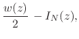 |
|||
 |
(63) |
and we must now write the integral ![]() explicitly in terms of
explicitly in terms of
![]() ,
, ![]() and
and ![]() ,
,
 |
|||
 |
|||
 |
(64) |
where
![]() and
and
![]() .
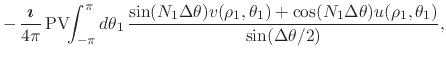
Once again we must rationalize the integrand, and using once more the
result shown in Equation (22) we get
.
Once again we must rationalize the integrand, and using once more the
result shown in Equation (22) we get
 |
|||
 |
|||
![$\displaystyle \frac{1}{4\pi}\,
\mbox{\rm PV}\!\!\int_{-\pi}^{\pi}d\theta_{1}\,
...
...ox{\boldmath$\imath$}
\sin(N_{1}\Delta\theta)
\right]
}
{\sin(\Delta\theta/2)},$](img242.png) |
(65) | ||
where
![]() and
and ![]() , with
, with
![]() . Expanding the numerator in the integrand of
this integral we have
. Expanding the numerator in the integrand of
this integral we have
| (66) | |||
and therefore we are left with the following expression for our integral,
 |
|||
 |
(67) | ||
where
![]() and
and ![]() , with
, with
![]() . Once again we note that, since by
construction the real and imaginary parts
. Once again we note that, since by
construction the real and imaginary parts
![]() and
and
![]() of
of
![]() for
for ![]() are
integrable real functions on the unit circle, and since there are no other
dependencies on
are
integrable real functions on the unit circle, and since there are no other
dependencies on ![]() in this equation, we may now take the
in this equation, we may now take the
![]() limit of this expression, in which the principal
value acquires its usual real meaning on the unit circle, thus obtaining
limit of this expression, in which the principal
value acquires its usual real meaning on the unit circle, thus obtaining
![$\displaystyle -\,
\frac{1}{4\pi}\,
\mbox{\rm PV}\!\!\int_{-\pi}^{\pi}d\theta_{1...
...{0em}{2ex}(N+1/2)\Delta\theta\right]
v(1,\theta_{1})
}
{\sin(\Delta\theta/2)}
+$](img250.png) |
|||
![$\displaystyle -\,
\frac{\mbox{\boldmath$\imath$}}{4\pi}\,
\mbox{\rm PV}\!\!\int...
...e{0em}{2ex}(N+1/2)\Delta\theta\right]
u(1,\theta_{1})
}
{\sin(\Delta\theta/2)},$](img251.png) |
(68) | ||
where
![]() and
and
![]() ,
in terms of which we now have the pair of equations at the unit circle
,
in terms of which we now have the pair of equations at the unit circle
 |
|||
 |
(69) |
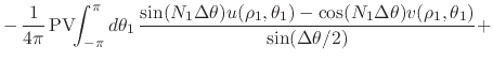
Using now the infinite collection of identities in
Equation (50) for the case ![]() , which allow us to
write
, which allow us to
write ![]() in terms of integrals similar to those in
in terms of integrals similar to those in
![]() ,
,
 | |||
![$\displaystyle \frac{1}{4\pi}\,
\mbox{\rm PV}\!\!\int_{-\pi}^{\pi}d\theta_{1}\,
...
...em}{2ex}(N+1/2)\Delta\theta\right]
v(1,\theta_{1})
}
{
\sin(\Delta\theta/2)
}
+$](img260.png) |
|||
![$\displaystyle +
\frac{\mbox{\boldmath$\imath$}}{4\pi}\,
\mbox{\rm PV}\!\!\int_{...
...0em}{2ex}(N+1/2)\Delta\theta\right]
u(1,\theta_{1})
}
{
\sin(\Delta\theta/2)
},$](img261.png) |
(70) | ||
where
![]() and
and
![]() ,
we may write for the complex partial sums
,
we may write for the complex partial sums
 |
|||
|
|||
![$\displaystyle +
\frac{\mbox{\boldmath$\imath$}}{4\pi}\,
\mbox{\rm PV}\!\!\int_{...
...em}{2ex}(N+1/2)\Delta\theta\right]
u(1,\theta_{1})
}
{
\sin(\Delta\theta/2)
}
+$](img264.png) |
|||
![$\displaystyle +
\frac{1}{4\pi}\,
\mbox{\rm PV}\!\!\int_{-\pi}^{\pi}d\theta_{1}\...
...{0em}{2ex}(N+1/2)\Delta\theta\right]
v(1,\theta_{1})
}
{\sin(\Delta\theta/2)}
+$](img265.png) |
|||
![$\displaystyle +
\frac{\mbox{\boldmath$\imath$}}{4\pi}\,
\mbox{\rm PV}\!\!\int_{...
...e{0em}{2ex}(N+1/2)\Delta\theta\right]
u(1,\theta_{1})
}
{\sin(\Delta\theta/2)}.$](img266.png) |
(71) | ||
As one can see in this equation, all the terms involving
![]() cancel off, and
therefore we are left with
cancel off, and
therefore we are left with
![$\displaystyle \frac{1}{2\pi}\,
\mbox{\rm PV}\!\!\int_{-\pi}^{\pi}d\theta_{1}\,
...
...em}{2ex}(N+1/2)\Delta\theta\right]
u(1,\theta_{1})
}
{
\sin(\Delta\theta/2)
}
+$](img268.png) |
|||
![$\displaystyle +
\frac{\mbox{\boldmath$\imath$}}{2\pi}\,
\mbox{\rm PV}\!\!\int_{...
...0em}{2ex}(N+1/2)\Delta\theta\right]
v(1,\theta_{1})
}
{
\sin(\Delta\theta/2)
},$](img269.png) |
(72) |
where
![]() and
and
![]() .
We now observe that, since by hypothesis
.
We now observe that, since by hypothesis ![]() is integrable on the
unit circle, the Cauchy principal value refers only to the possible
explicit non-integrable singularity of the integrands, due to the zero of
the denominators at
is integrable on the
unit circle, the Cauchy principal value refers only to the possible
explicit non-integrable singularity of the integrands, due to the zero of
the denominators at
![]() . However, since the numerators of
the integrands are also zero at that point, the integrands are not really
divergent at all at that point, so that from this point on we may drop the
principal value. We have therefore our final results for the real partial
sums, for both
. However, since the numerators of
the integrands are also zero at that point, the integrands are not really
divergent at all at that point, so that from this point on we may drop the
principal value. We have therefore our final results for the real partial
sums, for both ![]() and
and ![]() ,
,
![$\displaystyle \frac{1}{2\pi}\,
\int_{-\pi}^{\pi}d\theta_{1}\,
\frac
{
\sin\!\le...
...m}{2ex}(N+1/2)\Delta\theta\right]
}
{
\sin(\Delta\theta/2)
}\,
u(1,\theta_{1}),$](img272.png) |
|||
![$\displaystyle \frac{1}{2\pi}\,
\int_{-\pi}^{\pi}d\theta_{1}\,
\frac
{
\sin\!\le...
...m}{2ex}(N+1/2)\Delta\theta\right]
}
{
\sin(\Delta\theta/2)
}\,
v(1,\theta_{1}),$](img275.png) |
(73) |
where
![]() and
and
![]() .
These are the well-known results for the partial sums, in terms of
Dirichlet integrals [#!FSchurchill!#]. Note that the two equations above
have exactly the same form, which is to be expected, since the result
holds for all zero-average integrable real functions, including of course
both
.
These are the well-known results for the partial sums, in terms of
Dirichlet integrals [#!FSchurchill!#]. Note that the two equations above
have exactly the same form, which is to be expected, since the result
holds for all zero-average integrable real functions, including of course
both
![]() and
and
![]() . Therefore, given an
arbitrary zero-average integrable real function
. Therefore, given an
arbitrary zero-average integrable real function ![]() on the unit
circle, we have that the partial sums of its Fourier series are given by
on the unit
circle, we have that the partial sums of its Fourier series are given by
![\begin{displaymath}
S_{N}^{F}(\theta)
=
\frac{1}{2\pi}\,
\int_{-\pi}^{\pi}d\...
...\rule{0em}{2ex}(\theta_{1}-\theta)/2\right]}\,
f(\theta_{1}),
\end{displaymath}](img276.png) |
(74) |
where
![]() . Note that, although this result is
already very well known, we have showed here that it does follow from our
complex-analytic structure. This completes the proof of the first part of
Theorem 5.
. Note that, although this result is
already very well known, we have showed here that it does follow from our
complex-analytic structure. This completes the proof of the first part of
Theorem 5.
Once more, it is interesting to observe that this relation can be
interpreted as a linear integral operator acting on the space of
zero-average integrable real functions defined on the unit circle, this
time resulting in the ![]() partial sum of the Fourier series of a
zero-average integrable real function, a partial sum which is itself a
zero-average integrable real function. The integration kernel of this
integral operator
partial sum of the Fourier series of a
zero-average integrable real function, a partial sum which is itself a
zero-average integrable real function. The integration kernel of this
integral operator
![]() depends only on
depends only on ![]() and on the
difference
and on the
difference
![]() , and is given by
, and is given by
![\begin{displaymath}
K_{{\cal D}_{\rm s}}(N,\theta-\theta_{1})
=
\frac{1}{2\pi...
...]}
{\sin\!\left[\rule{0em}{2ex}(\theta_{1}-\theta)/2\right]},
\end{displaymath}](img278.png) |
(75) |
where
![]() , so that the action of the operator on
, so that the action of the operator on
![]() can be written as
can be written as
| (76) |
Considering that its kernel is given by a Dirichlet integral, one might
call this the Dirichlet operator, so that the ![]() partial
sum of the Fourier series of
partial
sum of the Fourier series of ![]() is given by the action of this
operator on the zero-average integrable real function
is given by the action of this
operator on the zero-average integrable real function ![]() ,
,
| (77) |
where
![]() . Note that
. Note that
![]() constitutes in fact a whole collection of linear integral operators acting
on the space of zero-average integrable real functions.
constitutes in fact a whole collection of linear integral operators acting
on the space of zero-average integrable real functions.
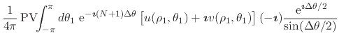
Using once more the very same elements that were used above for the complex partial sums, we may also write corresponding results for the complex remainders,
 |
|||
|
|||
|
|||
|
|||
![$\displaystyle -\,
\frac{\mbox{\boldmath$\imath$}}{4\pi}\,
\mbox{\rm PV}\!\!\int...
...e{0em}{2ex}(N+1/2)\Delta\theta\right]
u(1,\theta_{1})
}
{\sin(\Delta\theta/2)}.$](img283.png) |
(78) | ||
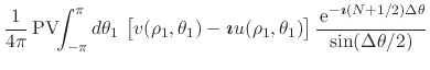
As one can see in this equation, this time all the terms involving
![]() chancel off, and
therefore we are left with
chancel off, and
therefore we are left with
![$\displaystyle \frac{1}{2\pi}\,
\mbox{\rm PV}\!\!\int_{-\pi}^{\pi}d\theta_{1}\,
...
...em}{2ex}(N+1/2)\Delta\theta\right]
v(1,\theta_{1})
}
{
\sin(\Delta\theta/2)
}
+$](img285.png) |
|||
![$\displaystyle -\,
\frac{\mbox{\boldmath$\imath$}}{2\pi}\,
\mbox{\rm PV}\!\!\int...
...0em}{2ex}(N+1/2)\Delta\theta\right]
u(1,\theta_{1})
}
{
\sin(\Delta\theta/2)
},$](img286.png) |
(79) |
where
![]() and
and
![]() .
We have therefore our results for the real remainders, for both
.
We have therefore our results for the real remainders, for both
![]() and
and ![]() ,
,
![$\displaystyle \frac{1}{2\pi}\,
\mbox{\rm PV}\!\!\int_{-\pi}^{\pi}d\theta_{1}\,
...
...m}{2ex}(N+1/2)\Delta\theta\right]
}
{
\sin(\Delta\theta/2)
}\,
v(1,\theta_{1}),$](img289.png) |
|||
![$\displaystyle -\,
\frac{1}{2\pi}\,
\mbox{\rm PV}\!\!\int_{-\pi}^{\pi}d\theta_{1...
...m}{2ex}(N+1/2)\Delta\theta\right]
}
{
\sin(\Delta\theta/2)
}\,
u(1,\theta_{1}),$](img292.png) |
(80) |
where
![]() and
and
![]() .
Recalling that
.
Recalling that
![]() and that
and that
![]() almost everywhere over the unit circle, this completes the proof of
Theorem 5.
almost everywhere over the unit circle, this completes the proof of
Theorem 5.
We believe that these are new results, written in terms of integrals which
are similar to the Dirichlet integrals, but not identical to them. Note
that the remainder of the series of ![]() is given as an integral
involving its Fourier-conjugate function
is given as an integral
involving its Fourier-conjugate function ![]() , and vice versa.
Therefore, we conclude that the convergence condition of the Fourier
series of a given real function does not depend directly on that function,
but only indirectly, through the properties of its Fourier-conjugate real
function.
, and vice versa.
Therefore, we conclude that the convergence condition of the Fourier
series of a given real function does not depend directly on that function,
but only indirectly, through the properties of its Fourier-conjugate real
function.
Since we know that these two real functions are related by the compact Hilbert transform, we may write these equations as
![$\displaystyle \frac{1}{2\pi}\,
\mbox{\rm PV}\!\!\int_{-\pi}^{\pi}d\theta_{1}\,
...
...ta\theta\right]
}
{
\sin(\Delta\theta/2)
}\,
{\cal H}_{\rm c}[u(1,\theta_{1})],$](img293.png) |
|||
![$\displaystyle \frac{1}{2\pi}\,
\mbox{\rm PV}\!\!\int_{-\pi}^{\pi}d\theta_{1}\,
...
...ta\theta\right]
}
{
\sin(\Delta\theta/2)
}\,
{\cal H}_{\rm c}[v(1,\theta_{1})],$](img294.png) |
(81) |
where
![]() and
and
![]() .
Note that the two results are now identical in form. Therefore, given an
arbitrary zero-average integrable real function
.
Note that the two results are now identical in form. Therefore, given an
arbitrary zero-average integrable real function ![]() on the unit
circle, we have our final result for the remainder of its Fourier series,
on the unit
circle, we have our final result for the remainder of its Fourier series,
![\begin{displaymath}
R_{N}^{F}(\theta)
=
\frac{1}{2\pi}\,
\mbox{\rm PV}\!\!\i...
...{
\sin(\Delta\theta/2)
}\,
{\cal H}_{\rm c}[f(\theta_{1})],
\end{displaymath}](img295.png) |
(82) |
where
![]() and
and
![]() .
.
Once again, it is interesting to observe that this relation can be
interpreted as a linear integral operator acting on the space of
integrable zero-average real functions defined on the unit circle. The
operator
![]() , acting on the compact Hilbert transform
, acting on the compact Hilbert transform
![]() of such a function, results in the
of such a function, results in the ![]() remainder of
the Fourier series of the original function
remainder of
the Fourier series of the original function ![]() , a remainder
which, if it exists at all, is itself a zero-average integrable real
function. The integration kernel of the integral operator depends only on
, a remainder
which, if it exists at all, is itself a zero-average integrable real
function. The integration kernel of the integral operator depends only on
![]() and on the difference
and on the difference
![]() , and is given by
, and is given by
where
![]() , so that the action of the operator on
an arbitrarily given zero-average integrable real function
, so that the action of the operator on
an arbitrarily given zero-average integrable real function ![]() can
be written as
can
be written as
| (84) |
This new operator, which we might refer to as the conjugate Dirichlet
operator, is similar to the Dirichlet operator, and is such that the
![]() remainder of the Fourier series of the real function
remainder of the Fourier series of the real function
![]() is given by the action of this operator on the
Fourier-conjugate function
is given by the action of this operator on the
Fourier-conjugate function ![]() of the real function
of the real function ![]() ,
,
| (85) |
where
![]() . Note once more that
. Note once more that
![]() constitutes in fact a whole collection of linear
integral operators acting on the space of zero-average integrable real
functions. Note also that, since by hypothesis
constitutes in fact a whole collection of linear
integral operators acting on the space of zero-average integrable real
functions. Note also that, since by hypothesis ![]() and
and ![]() are integrable on the unit circle, the Cauchy principal value refers only
to the explicit non-integrable singularity of the integration kernel at
are integrable on the unit circle, the Cauchy principal value refers only
to the explicit non-integrable singularity of the integration kernel at
![]() . In this operator notation we have therefore that the
remainder of the Fourier series of an arbitrarily given zero-average
integrable real function
. In this operator notation we have therefore that the
remainder of the Fourier series of an arbitrarily given zero-average
integrable real function ![]() is given by the composition of
is given by the composition of
![]() with
with
![]() ,
,
| (86) |
Note that, according to the inverse of the relation shown in Equation (42) we may write as well that
| (87) |
which constitutes an equivalent way to express the remainder of the
Fourier series of ![]() in terms of the function itself.
in terms of the function itself.
Finally note that, given the results obtained here for the partial sums and remainders of the Fourier series, the expressions in the infinite collection of identities shown in Equation (50) have now, in fact, the very simple interpretation that was alluded to there, since we now see that they can in fact be written as
| (88) |
where
![]() , a fact which greatly clarifies the
nature of that infinite collections of identities.
, a fact which greatly clarifies the
nature of that infinite collections of identities.
![\begin{displaymath}
K_{{\cal D}_{\rm c}}(N,\theta-\theta_{1})
=
\frac{1}{2\pi...
...]}
{\sin\!\left[\rule{0em}{2ex}(\theta_{1}-\theta)/2\right]},
\end{displaymath}](img297.png)