Next: An Infinite Collection of Up: Complex Analysis of Real Previous: The Compact Hilbert Transform
We will now determine the action of the compact Hilbert transform on the
elements of the Fourier basis of functions. The case of the constant
function, which constitutes the ![]() element of the basis, that is the
single member of the basis which is not a zero-average function, must be
examined in separate. We will now prove the following simple theorem.
element of the basis, that is the
single member of the basis which is not a zero-average function, must be
examined in separate. We will now prove the following simple theorem.
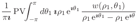
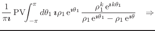
We start from the expression in Equation (17) for the very
simple case ![]() ,
,
| (29) |
where both ![]() and
and ![]() are on the circle
are on the circle ![]() of radius
of radius ![]() . We
may now write all quantities in this equation in terms of
. We
may now write all quantities in this equation in terms of ![]() ,
,
![]() and
and ![]() ,
,
 |
|||
 |
(30) |
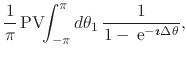
where
![]() . Note that, since there are no
remaining dependencies on
. Note that, since there are no
remaining dependencies on ![]() , we may now take the
, we may now take the
![]() limit of this expression, in which the principal value acquires
its usual real meaning on the unit circle. Just as in the previous
section, in order to identify separately the real and imaginary parts of
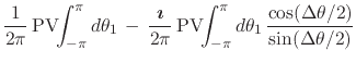
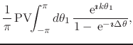
this equation, we must now rationalize the integrand. Using the result in
Equation (21) we obtain
limit of this expression, in which the principal value acquires
its usual real meaning on the unit circle. Just as in the previous
section, in order to identify separately the real and imaginary parts of
this equation, we must now rationalize the integrand. Using the result in
Equation (21) we obtain
![$\displaystyle \frac{1}{2\pi}\,
\mbox{\rm PV}\!\!\int_{-\pi}^{\pi}d\theta_{1}\,
...
...{\boldmath$\imath$}\,
\frac{\cos(\Delta\theta/2)}{\sin(\Delta\theta/2)}
\right]$](img127.png) |
|||
 |
|||
 |
(31) |
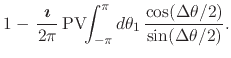
It follows therefore that we have
| (32) |
which is the statement that
![]() . Note that, since
. Note that, since
![]() , which in the context of this integral
implies that
, which in the context of this integral
implies that
![]() , by means of a trivial
transformation of variables this integral can also be shown to be zero by
simple parity arguments. Given the linearity of the compact Hilbert
transform, it is equally true that, for any real constant
, by means of a trivial
transformation of variables this integral can also be shown to be zero by
simple parity arguments. Given the linearity of the compact Hilbert
transform, it is equally true that, for any real constant ![]() , we have
that
, we have
that
![]() , so that all constant functions are mapped to the null
function. This completes the proof of Theorem 2.
, so that all constant functions are mapped to the null
function. This completes the proof of Theorem 2.
Let us now consider all the remaining elements of the Fourier basis of functions. We will prove the following theorem.
| (33) |
In order to prove this theorem we start from the expression in
Equation (17) for the case ![]() , where
, where
![]() , that is, for a strictly positive power of
, that is, for a strictly positive power of
![]() , which is therefore an inner analytic function. Note that these are
all the elements of the complex Taylor basis of functions, with the
exception of the constant function. We have therefore
, which is therefore an inner analytic function. Note that these are
all the elements of the complex Taylor basis of functions, with the
exception of the constant function. We have therefore
| (34) |
where both ![]() and
and ![]() are on the circle
are on the circle ![]() of radius
of radius ![]() . We
may now write all quantities in this equation in terms of
. We
may now write all quantities in this equation in terms of ![]() ,
,
![]() and
and ![]() ,
,
 |
|||
 |
(35) |
where
![]() . Note that, since there are no
remaining dependencies on
. Note that, since there are no
remaining dependencies on ![]() , we may now take the
, we may now take the
![]() limit of this expression, in which the principal value acquires
its usual real meaning on the unit circle. In the limit we have
limit of this expression, in which the principal value acquires
its usual real meaning on the unit circle. In the limit we have
| (36) |
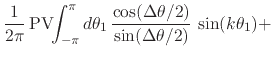
Just as in the previous cases, in order to identify separately the real and imaginary parts of this equation, we must now rationalize the integrand. Using the result in Equation (21) we obtain
![$\displaystyle \frac{1}{2\pi}\,
\mbox{\rm PV}\!\!\int_{-\pi}^{\pi}d\theta_{1}\,
...
...{\boldmath$\imath$}\,
\frac{\cos(\Delta\theta/2)}{\sin(\Delta\theta/2)}
\right]$](img100.png) |
|||
![$\displaystyle \frac{1}{2\pi}\,
\mbox{\rm PV}\!\!\int_{-\pi}^{\pi}d\theta_{1}\,
...
...}{2ex}
\cos(k\theta_{1})
+
\mbox{\boldmath$\imath$}
\sin(k\theta_{1})
\right]
+$](img145.png) |
|||
![$\displaystyle +
\frac{1}{2\pi}\,
\mbox{\rm PV}\!\!\int_{-\pi}^{\pi}d\theta_{1}\...
...m}{2ex}
\sin(k\theta_{1})
-
\mbox{\boldmath$\imath$}
\cos(k\theta_{1})
\right],$](img146.png) |
(37) | ||
where
![]() and
and
![]() .
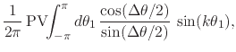
The first two integrals in the last form of the equation above are zero
for all
.
The first two integrals in the last form of the equation above are zero
for all ![]() because they are integrals of cosines and sines over integer
multiples of their periods, so that we may now separate the real and
imaginary parts of the remaining terms and thus get
because they are integrals of cosines and sines over integer
multiples of their periods, so that we may now separate the real and
imaginary parts of the remaining terms and thus get
 |
|||
 |
(38) |
where
![]() and
and
![]() .
We therefore obtain the action of the compact Hilbert transform on the
elements of the Fourier basis,
.
We therefore obtain the action of the compact Hilbert transform on the
elements of the Fourier basis,
 |
|||
 |
(39) |
where
![]() and
and
![]() .
The second equation above is the transform applied to the cosines and the
first equation is the inverse transform applied to the sines. As one can
see, the transform does indeed have the property of replacing cosines with
sines and sines with minus cosines, as expected. This completes the proof
of Theorem 3.
.
The second equation above is the transform applied to the cosines and the
first equation is the inverse transform applied to the sines. As one can
see, the transform does indeed have the property of replacing cosines with
sines and sines with minus cosines, as expected. This completes the proof
of Theorem 3.
One can now see that the application of the compact Hilbert transform to
the Fourier series of an arbitrarily given zero-average integrable real
function ![]() on the unit circle will produce the Fourier series of
its Fourier-conjugate real function
on the unit circle will produce the Fourier series of
its Fourier-conjugate real function ![]() . Given the linearity of
the transform, if we apply it to the Fourier series of
. Given the linearity of
the transform, if we apply it to the Fourier series of ![]() we get
we get
![$\displaystyle {\cal H}_{\rm c}\!\left\{
\sum_{k=1}^{\infty}
\left[
\rule{0em}{2ex}
\alpha_{k}\cos(k\theta)
+
\beta_{k}\sin(k\theta)
\right]
\right\}$](img155.png) |
![$\displaystyle \sum_{k=1}^{\infty}
\left\{
\rule{0em}{2.5ex}
\alpha_{k}
{\cal H}...
...
\beta_{k}
{\cal H}_{\rm c}\!\left[\rule{0em}{2ex}\sin(k\theta)\right]
\right\}$](img156.png) |
||
![$\displaystyle \sum_{k=1}^{\infty}
\left[
\rule{0em}{2ex}
\alpha_{k}
\sin(k\theta)
-
\beta_{k}
\cos(k\theta)
\right],$](img157.png) |
(40) |
where this last one is the Fourier series of the real function
![]() , which is the Fourier conjugate of
, which is the Fourier conjugate of ![]() . Hence, if
. Hence, if
![]() is the complex power series given in
Equation (6), if
is the complex power series given in
Equation (6), if
![]() is the
Fourier series of
is the
Fourier series of ![]() and
and
![]() is
the Fourier series of
is
the Fourier series of ![]() , then we have that
, then we have that
| (41) |
Note that the same is true for the corresponding partial sums, as well as
for the corresponding remainders, so long as the latter exist at all. If
![]() is the
is the ![]() partial sum and
partial sum and
![]() is the
is the ![]() remainder of the complex power
series given in Equation (6), and if
remainder of the complex power
series given in Equation (6), and if
![]() is the
is the ![]() partial sum
of the real Fourier series of
partial sum
of the real Fourier series of ![]() , if
, if
![]() is the
is the ![]() partial sum
of the Fourier series of
partial sum
of the Fourier series of ![]() , if
, if
![]() is the
is the ![]() remainder
of the Fourier series of
remainder
of the Fourier series of ![]() and if
and if
![]() is the
is the ![]() remainder
of the Fourier series of
remainder
of the Fourier series of ![]() , then we have
, then we have
Of course, in each one of these cases the inverse mapping holds as well,
using the inverse transform to take us from the quantities related to
![]() back to the corresponding quantities related to
back to the corresponding quantities related to ![]() .
.
![$\displaystyle {\cal H}_{\rm c}\!\left[\rule{0em}{2ex}S_{N}^{F,f}(\theta)\right],$](img170.png)
![$\displaystyle {\cal H}_{\rm c}\!\left[\rule{0em}{2ex}R_{N}^{F,f}(\theta)\right].$](img172.png)