Next: Action on the Fourier Up: Complex Analysis of Real Previous: Review of Real Functions
Let ![]() be an integrable real function on
be an integrable real function on ![]() , with
Fourier coefficients as given in Equation (4). As was
shown in [#!CAoRFIII!#] the real function
, with
Fourier coefficients as given in Equation (4). As was
shown in [#!CAoRFIII!#] the real function
![]() which
is the Fourier-conjugate function to
which
is the Fourier-conjugate function to
![]() has the same
Fourier coefficients, but with the meanings of
has the same
Fourier coefficients, but with the meanings of ![]() and
and
![]() interchanged, as shown in Equation (8). The
relations in Equations (4) and (8) can be
understood as the following collection of integral identities satisfied by
all pairs of Fourier-conjugate integrable real functions,
interchanged, as shown in Equation (8). The
relations in Equations (4) and (8) can be
understood as the following collection of integral identities satisfied by
all pairs of Fourier-conjugate integrable real functions,
 |
 |
||
 |
 |
(10) |
for
![]() . It is well known that this replacement
of
. It is well known that this replacement
of ![]() with
with ![]() and of
and of ![]() with
with
![]() can be effected by the use of the Hilbert transform.
However, that transform was originally introduced by Hilbert for real
functions defined on the whole real line, rather that on the unit circle
as is our case here. Therefore, the first thing that we will do here is to
define a compact version of the Hilbert transform that applies to real
functions defined on the unit circle.
can be effected by the use of the Hilbert transform.
However, that transform was originally introduced by Hilbert for real
functions defined on the whole real line, rather that on the unit circle
as is our case here. Therefore, the first thing that we will do here is to
define a compact version of the Hilbert transform that applies to real
functions defined on the unit circle.
Since the Fourier coefficient ![]() of
of ![]() has no effect on
the definition of the Fourier-conjugate function
has no effect on
the definition of the Fourier-conjugate function ![]() , and in order
for this pair of real functions to be related in a unique way, we will
assume that
, and in order
for this pair of real functions to be related in a unique way, we will
assume that ![]() is also a zero-average real function,
is also a zero-average real function,
| (11) |
thus implying for its ![]() Fourier coefficient that
Fourier coefficient that ![]() . This
does not affect, of course, any subsequent arguments about the convergence
of the Fourier series. According to the construction presented
in [#!CAoRFI!#] and reviewed in Section 2, from the other
Fourier coefficients
. This
does not affect, of course, any subsequent arguments about the convergence
of the Fourier series. According to the construction presented
in [#!CAoRFI!#] and reviewed in Section 2, from the other
Fourier coefficients ![]() and
and ![]() , for
, for
![]() , we may construct the complex coefficients
, we may construct the complex coefficients
![]() , for
, for
![]() , where
we now have
, where
we now have ![]() , and from these we may construct the corresponding
inner analytic function
, and from these we may construct the corresponding
inner analytic function ![]() shown in Equation (7),
which is now, in fact, a proper inner analytic function, since
shown in Equation (7),
which is now, in fact, a proper inner analytic function, since
![]() implies that
implies that ![]() .
.
Since
![]() and
and
![]() are harmonic conjugate
functions to each other, it is now clear that there is a one-to-one
correspondence between
are harmonic conjugate
functions to each other, it is now clear that there is a one-to-one
correspondence between
![]() and
and
![]() , and in
particular between
, and in
particular between ![]() and
and ![]() . Therefore, there is a
one-to-one correspondence between
. Therefore, there is a
one-to-one correspondence between ![]() and
and ![]() , in this
case valid almost everywhere on the unit circle, since we have shown
in [#!CAoRFI!#] that
, in this
case valid almost everywhere on the unit circle, since we have shown
in [#!CAoRFI!#] that
![]() and that
and that
![]() , both almost everywhere over the unit circle.
Therefore, a transformation must exist that produces
, both almost everywhere over the unit circle.
Therefore, a transformation must exist that produces ![]() from
from
![]() almost everywhere over the unit circle, as well as an inverse
transformation that recovers
almost everywhere over the unit circle, as well as an inverse
transformation that recovers ![]() from
from ![]() almost
everywhere over the unit circle. In this section we will show that the
following definition accomplishes this.
almost
everywhere over the unit circle. In this section we will show that the
following definition accomplishes this.
If ![]() is an arbitrarily given zero-average integrable real
function defined on the unit circle, then its compact Hilbert
transform
is an arbitrarily given zero-average integrable real
function defined on the unit circle, then its compact Hilbert
transform ![]() is the real function defined by
is the real function defined by
![$\displaystyle -\,
\frac{1}{2\pi}\,
\mbox{\rm PV}\!\!\int_{-\pi}^{\pi}d\theta_{1...
...ht]}
{\sin\!\left[\rule{0em}{2ex}(\theta_{1}-\theta)/2\right]}\,
f(\theta_{1}),$](img61.png) |
(12) |
where
![]() stands for the Cauchy principal value, and where
stands for the Cauchy principal value, and where
![]() is the notation we will use for the compact Hilbert
transform applied to the real function
is the notation we will use for the compact Hilbert
transform applied to the real function ![]() .
.
We will now prove the following theorem.
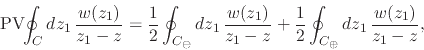
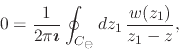
In order to derive these facts from our complex-analytic structure, we
start from the Cauchy integral formula for the inner analytic function
![]() ,
,
where ![]() can be taken as a circle centered at the origin, with radius
can be taken as a circle centered at the origin, with radius
![]() , and where we write
, and where we write ![]() and
and ![]() in polar coordinates as
in polar coordinates as
![]() and
and
![]() . The
integral formula in Equation (13) is valid for
. The
integral formula in Equation (13) is valid for
![]() , and in fact, by the Cauchy-Goursat theorem, the integral
is zero if
, and in fact, by the Cauchy-Goursat theorem, the integral
is zero if ![]() , since both
, since both ![]() and
and ![]() are within the open
unit disk, a region where
are within the open
unit disk, a region where ![]() is analytic. We must now determine what
happens if
is analytic. We must now determine what
happens if ![]() , that is, if
, that is, if ![]() is on the circle
is on the circle ![]() of radius
of radius
![]() . Note that in this case we may slightly deform the integration
contour
. Note that in this case we may slightly deform the integration
contour ![]() in order to have it pass on one side or the other of the
simple pole of the integrand at
in order to have it pass on one side or the other of the
simple pole of the integrand at ![]() . If we use a deformed contour
. If we use a deformed contour
![]() that excludes the pole from its interior, then we
have, instead of Equation (13),
that excludes the pole from its interior, then we
have, instead of Equation (13),
due to the Cauchy-Goursat theorem, while if we use a deformed contour
![]() that includes the pole in its interior, then we have,
just as in Equation (13),
that includes the pole in its interior, then we have,
just as in Equation (13),
Since by the Sokhotskii-Plemelj theorem [#!sokhplem!#] the Cauchy
principal value of the integral over the circle ![]() is the arithmetic
average of these two integrals, in the limit where the deformations
vanish, a limit which does not really have to be considered in detail, so
long as the deformations do not cross any other singularities,
is the arithmetic
average of these two integrals, in the limit where the deformations
vanish, a limit which does not really have to be considered in detail, so
long as the deformations do not cross any other singularities,
 |
(16) |
adding Equations (14) and (15) we may conclude that
where we now have ![]() , that is, both
, that is, both ![]() and
and ![]() are on
the circle
are on
the circle ![]() of radius
of radius ![]() within the open unit disk. This
formula can be understood as a special version of the Cauchy integral
formula, and will be used repeatedly in what follows. We may now write all
quantities in this equation in terms of the polar coordinates
within the open unit disk. This
formula can be understood as a special version of the Cauchy integral
formula, and will be used repeatedly in what follows. We may now write all
quantities in this equation in terms of the polar coordinates ![]() ,
,
![]() and
and ![]() ,
,
 |
|||
 |
(18) |
where
![]() . Note that, since by construction
the real and imaginary parts
. Note that, since by construction
the real and imaginary parts
![]() and
and
![]() of
of
![]() for
for ![]() are integrable real functions on
the unit circle, and since there are no other dependencies on
are integrable real functions on
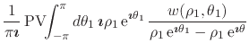
the unit circle, and since there are no other dependencies on ![]() in this expression, we may now take the
in this expression, we may now take the
![]() limit of
this equation, in which the principal value acquires its usual real
meaning over the unit circle, that is, the meaning that the asymptotic
limits of the integral on either side of a non-integrable singularity must
be taken in the symmetric way. In that limit we have
limit of
this equation, in which the principal value acquires its usual real
meaning over the unit circle, that is, the meaning that the asymptotic
limits of the integral on either side of a non-integrable singularity must
be taken in the symmetric way. In that limit we have
In order to identify separately the real and imaginary parts of this equation, we must now rationalize the integrand of the integral shown. We will use the fact that
 |
 |
||
![$\displaystyle \frac
{
\left[
\rule{0em}{2ex}
1
-
\cos(\Delta\theta)
\right]
-
\mbox{\boldmath$\imath$}
\sin(\Delta\theta)
}
{
2-2\cos(\Delta\theta)
}$](img95.png) |
|||
![$\displaystyle \frac{1}{2}
\left[
1
-
\mbox{\boldmath$\imath$}\,
\frac
{
\sin(\Delta\theta)
}
{
1-\cos(\Delta\theta)
}
\right].$](img96.png) |
(20) |
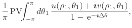
Using the half-angle trigonometric identities we may also write this result as
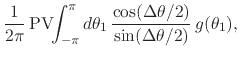
Using the result shown in Equation (21) back in Equation (19) we obtain
![$\displaystyle \frac{1}{2\pi}\,
\mbox{\rm PV}\!\!\int_{-\pi}^{\pi}d\theta_{1}\,
...
...{\boldmath$\imath$}\,
\frac{\cos(\Delta\theta/2)}{\sin(\Delta\theta/2)}
\right]$](img100.png) |
|||
![$\displaystyle \frac{1}{2\pi}\,
\mbox{\rm PV}\!\!\int_{-\pi}^{\pi}d\theta_{1}\,
...
...{0em}{2ex}
u(1,\theta_{1})
+
\mbox{\boldmath$\imath$}
v(1,\theta_{1})
\right]
+$](img101.png) |
|||
![$\displaystyle +
\frac{1}{2\pi}\,
\mbox{\rm PV}\!\!\int_{-\pi}^{\pi}d\theta_{1}\...
...e{0em}{2ex}
v(1,\theta_{1})
-
\mbox{\boldmath$\imath$}
u(1,\theta_{1})
\right].$](img102.png) |
(23) |
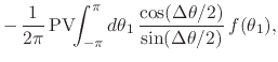
Since both
![]() and
and
![]() are zero-average real
functions on the unit circle, the first two integrals in the last form of
the equation above are zero, so that separating the real and imaginary
parts within this expression we are left with
are zero-average real
functions on the unit circle, the first two integrals in the last form of
the equation above are zero, so that separating the real and imaginary
parts within this expression we are left with
 |
|||
 |
(24) |
where
![]() . Separating the real and imaginary
parts of this equation we may now write that
. Separating the real and imaginary
parts of this equation we may now write that
 |
|||
 |
(25) |
where
![]() . Recalling that
. Recalling that
![]() and
and
![]() , almost everywhere on
the unit circle, we have
, almost everywhere on
the unit circle, we have
 |
|||
 |
(26) |
two equations which are thus valid almost everywhere as well. These are
the transformations relating the pair of Fourier-conjugate functions
![]() and
and ![]() . The second expression defines the compact
Hilbert transformation of
. The second expression defines the compact
Hilbert transformation of ![]() into
into ![]() , and the first one
defines the inverse transformation, which recovers
, and the first one
defines the inverse transformation, which recovers ![]() from
from
![]() . Note that in this notation the transform is defined with an
explicit minus sign, and that its inverse is simply minus the transform
itself,
. Note that in this notation the transform is defined with an
explicit minus sign, and that its inverse is simply minus the transform
itself,
![]() . This completes the proof of
Theorem 1.
. This completes the proof of
Theorem 1.
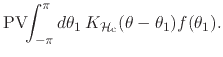
It is interesting to observe that this transform can be interpreted as a
linear integral operator acting on the space of zero-average integrable
real functions defined on the unit circle. The integration kernel of the
integral operator depends only on the difference
![]() , and
is given by
, and
is given by
so that the action of the operator on an arbitrarily given zero-average
real integrable function ![]() on the unit circle can be written as
on the unit circle can be written as
 |
(28) |
The operator is linear, invertible, and the composition of the operator
with itself results in the operation of multiplication by ![]() . Note that,
since by hypothesis
. Note that,
since by hypothesis ![]() is integrable on the unit circle, the
Cauchy principal value refers only to the explicit non-integrable
singularity of the integration kernel at the position
is integrable on the unit circle, the
Cauchy principal value refers only to the explicit non-integrable
singularity of the integration kernel at the position
![]() .
.
![$\displaystyle \frac{1}{2}
\left[
1
-
\mbox{\boldmath$\imath$}\,
\frac{\cos(\Delta\theta/2)}{\sin(\Delta\theta/2)}
\right]$](img97.png)
![\begin{displaymath}
K_{{\cal H}_{\rm c}}(\theta-\theta_{1})
=
-\,
\frac{1}{2...
...]}
{\sin\!\left[\rule{0em}{2ex}(\theta_{1}-\theta)/2\right]},
\end{displaymath}](img116.png)