Application in Partial Differential Equations

Let us now describe how one can use the low-pass filters in boundary value problems involving partial differential equations. The basic idea is that, if the solution of a boundary value problem leads to a divergent Fourier series for some physical quantity, then the correct physical interpretation of this fact is that the mathematical description of the physical system being dealt with lacks sufficient realism. This is usually a problem contained within the initial conditions used, or within the boundary conditions used, or both. The divergences are always consequences of singularities contained within these conditions. We therefore use the filters in order to smooth out the initial or boundary conditions, using some small range parameter $\varepsilon$ which is suggested by the relevant physical scales of the physical system. Having done that, we may then repeat the whole resolution of the boundary value problem. The solution obtained in this way will then present lesser convergence problems, and quite probably none at all.

While using this technique, it is useful to keep in mind some basic mathematical and physical facts regarding divergences and singularities. There are two basic types of divergence that can happen in a Fourier series, divergence to infinity and indefinite oscillations or endless wandering. If the series diverges everywhere over its periodic domain, then the divergences may occur for two reasons, either there may exist no real function that gives the Fourier coefficients of that series, or there may be a failure of the internal mathematical machinery to represent correctly an existing real function. On the other hand, if there is convergence almost everywhere, and only one or more isolated points of divergence to infinity, then it is likely that the divergences are caused by the real function actually having integrable singularities at these isolated points.

Only very radical divergence at all points within the domain can possibly imply the actual non-existence of a real function that gives the coefficients of the series. This is discussed in [2] and [3], in terms of an analytic structure that leads to a simple and natural classification of divergences and singularities. The typical case would be that in which the coefficients of a trigonometric series diverge exponentially with $k$ when $k\to\infty$, in which case the trigonometric series may fail to be a Fourier series at all. This is seldom the case, so that in general we have either oscillatory divergence almost everywhere, signifying a failure of the internal mathematical machinery to represent faithfully an existing real function, or divergence to infinity at isolated points where the real function being represented by the Fourier series has actual integrable singularities.

In strict physical terms every divergence represents a failure to represent or describe the physical world adequately. This means that either the fundamental physical theory being used has failed, or that the mathematical representation of the particular physical system at hand is inadequate. The latter is much more often the case than the former, with the description of the system being usually either oversimplified or incomplete. For well-established fundamental physical theories being used in a well-established domain of validity, the possibility of a fundamental failure of the theory is an extremely remote one. On the other hand, oversimplification of initial or boundary conditions is a relatively common occurrence.

It is often possible to greatly simplify the use of the filters, avoiding the necessity to solve the boundary value problem all over again after the application of the filter. This is a consequence of the fact that the filter operation often commutes with the differential operator contained within the partial differential equation. In order to see this, let us recall that the first-order filter can be understood as an integral operator, which acts on the space of integrable real functions, since it maps each real function to another real function. Let us show that the elements of the Fourier basis are eigenfunctions of this operator. If we apply the filter as defined in Equation (1) to one of the cosine functions of the basis we get

$$\begin{eqnarray*} \frac{1}{2\varepsilon} \int_{x-\varepsilon}^{x+\varepsilon}d... ...[ \frac{\sin(k\varepsilon)}{(k\varepsilon)} \right] \cos(kx). \end{eqnarray*}$$

This establishes the result, and also determines the eigenvalue, given by the ratio shown within brackets. Once again we see here the sinc function of the variable $(k\varepsilon)$, the same that appears in the Fourier expansions of the kernels. The same can be done for the sine functions, yielding

$$\begin{eqnarray*} \frac{1}{2\varepsilon} \int_{x-\varepsilon}^{x+\varepsilon}d... ...[ \frac{\sin(k\varepsilon)}{(k\varepsilon)} \right] \sin(kx). \end{eqnarray*}$$

Note that this establishes the fact that these are the eigenfunctions of the filter operator for all values of $\varepsilon$ in $(0,\pi)$. In other words, this fact is stable by small variations of the real parameter $\varepsilon$. As one can see, we have here the same eigenvalue as in the previous case. There is therefore a degenerescence between each pair of elements of the basis with the same value of $k$. It is also possible to show that, up to this degenerescence, and assuming the stability by small changes of $\varepsilon$, the elements of the Fourier basis are the only eigenfunctions of the filter operator when defined within the periodic interval, as one can see in Section A.13 of Appendix A. What all this means is that the filter acts in an extremely simple way on the Fourier expansions. If we have the Fourier expansion of the real function $f(x)$ in the periodic interval $[-\pi ,\pi ]$,

$$f(x) = \frac{1}{2}\, \alpha_{0} + \sum_{k=1}^{\infty} \left[ \alpha_{k}\cos(kx) + \beta_{k}\sin(kx) \right],$$

it follows at once that the corresponding expansion for the filtered function is

$$f_{\varepsilon}(x) = \frac{1}{2}\, \alpha_{0} + \sum_{... ...n(k\varepsilon)}{(k\varepsilon)} \right] \sin(kx) \right\}.$$

What this means is that the Fourier coefficients $\alpha_{\varepsilon,k}$ and $\beta_{\varepsilon,k}$ of $f_{\varepsilon}(x)$ are given by

$$\begin{eqnarray*} \alpha_{\varepsilon,k} & = & \left[ \frac{\sin(k\varepsilo... ... \frac{\sin(k\varepsilon)}{(k\varepsilon)} \right] \beta_{k}, \end{eqnarray*}$$

a fact that can be shown directly and independently of the operator-based argument used here, as one can see in Section A.12 of Appendix A. Since the $\sin(k\varepsilon)$ in the numerator of the ratio within brackets is a limited function, while in the denominator we have simply $(k\varepsilon)$, in terms of the asymptotic behavior of the coefficients the inclusion of the ratio, and hence the action of the filter, corresponds simply to the inclusion of a factor of $k$ in the denominator.

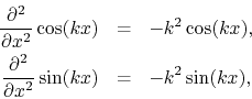
Since the elements of the Fourier basis are also eigenfunctions of the second-derivative operator, as one can easily see by simply calculating the derivatives,

$$\begin{eqnarray*} \frac{\partial^{2}}{\partial x^{2}}\cos(kx) & = & -k^{2}\co... ...ac{\partial^{2}}{\partial x^{2}}\sin(kx) & = & -k^{2}\sin(kx), \end{eqnarray*}$$

we may conclude that within the periodic interval the second-derivative operator and the first-order low-pass filter operator have a complete set of functions as a common set of eigenfunctions. It follows that the two operators commute, a result which can be immediately extended to the higher-order filters. Therefore, given any partial differential equation which is purely second-order on the variable $x$ on which the filter acts, and whose coefficients do not depend on that variable, it follows that if a function $f(x)$ solves the equation, then the filtered function $f_{\varepsilon}(x)$ is also a solution.

This leads to the fact that one may apply the filter directly to the solution of the unfiltered problem, thus obtaining the same result that one would obtain by first applying the filter to the initial or boundary conditions and then solving the boundary value problem all over again. This is the case for the Laplace equation, the wave equation and the diffusion equation, in either Cartesian or cylindrical coordinates. Since the unfiltered solution is represented in terms of a (possibly divergent) Fourier series, in such circumstances it is immediate to write down the filtered solution, by simply plugging the filter factor given by the sinc function into the coefficients of the Fourier series obtained in the usual way, as is illustrated by the examples in Appendix B. Since it usually takes much more work to solve the boundary value problem with the filtered initial or boundary conditions than to solve the corresponding unfiltered problem, this can save a lot of work and effort.