Next: Higher-Order Filters Up: Low-Pass Filters, Fourier Series Previous: Introduction
The low-pass filters are defined as operations on real functions leading
to other related real functions. Let us define the simplest such filter,
namely the first-order linear low-pass filter. Given a real function
![]() on the real line of the coordinate
on the real line of the coordinate ![]() , of which we require no more
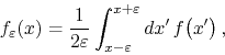
than that it be integrable, we define from it a filtered function
, of which we require no more
than that it be integrable, we define from it a filtered function
![]() by
by
where ![]() is a strictly positive real constant, usually meant to
be small by comparison to some physical scale, and which we will refer to
as the range of the filter. One can also define
is a strictly positive real constant, usually meant to
be small by comparison to some physical scale, and which we will refer to
as the range of the filter. One can also define ![]() by
continuity, as the
by
continuity, as the
![]() limit of this expression, which is
mostly but not always identical to
limit of this expression, which is
mostly but not always identical to ![]() . The transition from
. The transition from ![]() to
to
![]() constitutes an operation within the space of real
functions. A discrete version of this operation is known in numerical and
graphical settings as that of taking running averages. Another
similar operation is known in quantum field theory as block
renormalization. What we do here is to map the value of
constitutes an operation within the space of real
functions. A discrete version of this operation is known in numerical and
graphical settings as that of taking running averages. Another
similar operation is known in quantum field theory as block
renormalization. What we do here is to map the value of ![]() at
at ![]() to its average value over a symmetric interval around
to its average value over a symmetric interval around ![]() . This results in
a new real function
. This results in
a new real function
![]() that is smoother than the
original one, since the filter clearly damps out the high-frequency
components of the Fourier spectrum of
that is smoother than the
original one, since the filter clearly damps out the high-frequency
components of the Fourier spectrum of ![]() , as will be shown explicitly
in what follows.
, as will be shown explicitly
in what follows.
The filter can be understood as a linear integral operator acting in the
space of integrable real functions. It may be written as an integral over
the whole real line involving a kernel
![]() with compact support,
with compact support,
where the kernel is defined as
![]() for
for
![]() , and as
, and as
![]() for
for
![]() . This kernel is a discontinuous even function of
. This kernel is a discontinuous even function of
![]() that has unit integral. If the functions one is
dealing with are defined in a periodic interval such as
that has unit integral. If the functions one is
dealing with are defined in a periodic interval such as ![]() , then
the integral above has to be restricted to that interval, and the kernel
can be easily expressed in terms of a convergent Fourier series,
, then
the integral above has to be restricted to that interval, and the kernel
can be easily expressed in terms of a convergent Fourier series,
![\begin{displaymath}
K_{\varepsilon}\!\left(x-x'\right)
=
\frac{1}{2\pi}
+
\...
...\varepsilon)}
\right]
\cos\!\left[k\left(x-x'\right)\right],
\end{displaymath}](img21.png)
where we assume that
![]() . The calculation of the
coefficients of this series is completely straightforward. The series can
be shown to be convergent by the Dirichlet test, or alternatively by the
monotonicity criterion discussed in [3]. The quantity within
square brackets is known as the sinc function of the variable
. The calculation of the
coefficients of this series is completely straightforward. The series can
be shown to be convergent by the Dirichlet test, or alternatively by the
monotonicity criterion discussed in [3]. The quantity within
square brackets is known as the sinc function of the variable
![]() . In spite of appearances, it is an analytic function,
assuming the value
. In spite of appearances, it is an analytic function,
assuming the value ![]() at zero.
at zero.
Although it is possible to define the filter of range ![]() inside
a periodic interval even if the overall range is larger that the length of
the interval, that is when
inside
a periodic interval even if the overall range is larger that the length of
the interval, that is when
![]() in our case here, there is
little point in doing so. The central idea of the filter is that the range
be small compared to the relevant scales of a given problem, and once a
periodic interval is introduces it immediately establishes such a scale
with its length. Therefore we should have at least
in our case here, there is
little point in doing so. The central idea of the filter is that the range
be small compared to the relevant scales of a given problem, and once a
periodic interval is introduces it immediately establishes such a scale
with its length. Therefore we should have at least
![]() ,
and more often
,
and more often
![]() . We will therefore adopt as a basic
hypothesis, from now on, the condition that the range be smaller than the
length of the periodic interval, whenever we work with periodic functions
within such an interval.
. We will therefore adopt as a basic
hypothesis, from now on, the condition that the range be smaller than the
length of the periodic interval, whenever we work with periodic functions
within such an interval.
The filter defined above has several interesting properties, which are the
reasons for its usefulness. Some of the most important and basic ones
follow. In every case it is clear that ![]() must be an integrable
function, otherwise it is not even possible to define the corresponding
filtered function.
must be an integrable
function, otherwise it is not even possible to define the corresponding
filtered function.
Only lower powers of ![]() with the same parity as
with the same parity as ![]() appear in this
polynomial. All the other coefficients contain strictly positive powers
of
appear in this
polynomial. All the other coefficients contain strictly positive powers
of
![]() , and thus tend to zero when
, and thus tend to zero when
![]() .
This means that in the
.
This means that in the
![]() limit the filter becomes the
identity, in so far as polynomials are concerned.
limit the filter becomes the
identity, in so far as polynomials are concerned.
Up to this point we have assumed that ![]() is defined on the whole real
line. If instead of this it is defined within a periodic interval, then we
have a few more properties.
is defined on the whole real
line. If instead of this it is defined within a periodic interval, then we
have a few more properties.
![\begin{eqnarray*}
\alpha_{\varepsilon,k}
& = &
\left[
\frac{\sin(k\varepsilo...
... \frac{\sin(k\varepsilon)}{(k\varepsilon)}
\right]
\beta_{k}.
\end{eqnarray*}](img36.png)
Once more we see here the presence of the sinc function of the variable
![]() .
.
All these properties can be demonstrated directly on the real line, and
some such demonstrations can be found in Appendix A. For
our purposes here one of the most important properties is the last one,
since it implies that the action of the filter, when represented in the
Fourier series of the real function, is very simple and has the effect of
rendering the filtered series more rapidly convergent than the original
one, since the filtered coefficients contain an extra factor of ![]() and
hence approach zero faster than the original ones as we make
and
hence approach zero faster than the original ones as we make ![]() .
.
The usefulness of the filter in physics applications, and the very possibility of using it to regularize divergent Fourier series in such circumstances, stem from two facts related to the mathematical representation of nature in physics. First, such a representation is always an approximate one. All physical measurements, as well as all theoretical calculations, of quantities which are represented by continuous variables, can only be performed with a finite amount of precision, that is, within finite and non-zero errors. In fact, not only this is true in practice, but with the advent of relativistic quantum mechanics and quantum field theory, it became a limitation in principle as well. Second, all physical laws are valid within a certain range of length, time or energy scales. Given any physical measurements or theoretical calculations, there is always a length or time scale below which, or an energy scale above which, the measurements and calculation, as well as the hypotheses behind them, cease to have any meaning.
If we observe that the application of a filter with range parameter
![]() appreciably changes the function, and therefore the
representation of nature that it implements, only at scales of the order
of
appreciably changes the function, and therefore the
representation of nature that it implements, only at scales of the order
of ![]() or smaller, while at the same time resulting in series
with better convergence characteristics for all non-zero values of
or smaller, while at the same time resulting in series
with better convergence characteristics for all non-zero values of
![]() , no matter how small, it becomes clear that it is always
possible to choose
, no matter how small, it becomes clear that it is always
possible to choose ![]() small enough so that no appreciable
change in the physics is entailed within the relevant scales. We conclude
therefore that it is always possible to filter the real functions involved
in physics applications, in order to have a representation of the physics
in terms of convergent series, without the introduction of any physically
relevant changes in the description of nature and its laws. In fact, many
times it turns out that the introduction of the low-pass filter actually
improves the approximate representation of nature used in the
applications, rather than harming it in any way, as shown in the examples
discussed in Appendix B.
small enough so that no appreciable
change in the physics is entailed within the relevant scales. We conclude
therefore that it is always possible to filter the real functions involved
in physics applications, in order to have a representation of the physics
in terms of convergent series, without the introduction of any physically
relevant changes in the description of nature and its laws. In fact, many
times it turns out that the introduction of the low-pass filter actually
improves the approximate representation of nature used in the
applications, rather than harming it in any way, as shown in the examples
discussed in Appendix B.