Next: Final Component Equation Up: Extension of the Schwarzschild Previous: Solution in Vacuum
We will now describe a method for obtaining the solution in the presence
of fluid matter. We start with an informed guess about the form of the
function ![]() . The ansatz that we will present here is suggested
by the well-known Jebsen-Birkhoff [#!JebsenTheorem!#,#!BirkhoffTheorem!#]
theorem, which states that any spherically symmetric solution of the
vacuum field equation must be both static and asymptotically flat, and
therefore must be given by the Schwarzschild metric. It is to be noted,
however, that this very statement implies, as a matter of course, that the
solution at issue lies in a region that has continuous access to radial
infinity.
. The ansatz that we will present here is suggested
by the well-known Jebsen-Birkhoff [#!JebsenTheorem!#,#!BirkhoffTheorem!#]
theorem, which states that any spherically symmetric solution of the
vacuum field equation must be both static and asymptotically flat, and
therefore must be given by the Schwarzschild metric. It is to be noted,
however, that this very statement implies, as a matter of course, that the
solution at issue lies in a region that has continuous access to radial
infinity.
It is usually stated that the theorem also implies that the geometry
within the vacuous region between two spherically symmetric concentric
shells, which do not need to be thin, is given by a radial section of the
Schwarzschild solution, with the corresponding internal mass, between the
corresponding two radii. However, this is not entirely correct, as one can
see in the discussion presented in [#!JBTheoremError!#]. While it is
correct for the spatial part of the geometry, there is a change in
the temporal part. This can be seen in simple terms if one realizes
that there must be a red-shift/blue-shift relationship between the
internal bounded vacuous region and the external region at radial
infinity. In order to see this it suffices to consider a monochromatic
beam of light propagating from radial infinity towards the localized
matter distribution, and passing through a thin radial hole made across
the outer shell, into the bounded vacuous region. It is quite clear that
the blue shift undergone by this beam of light is not the same
that one would get in the absence of the outer shell, since it includes
the blue-shift effect of the mass in the outer shell. Therefore, the
coefficient ![]() of the term
of the term ![]() of the invariant
interval, which gives this blue shift, must differ from the one in the
Schwarzschild solution for the internal mass.
of the invariant
interval, which gives this blue shift, must differ from the one in the
Schwarzschild solution for the internal mass.
In short, we may safely assume that the Jebsen-Birkhoff theorem does have
the interesting consequence that the geometry within a spherically
symmetric empty shell of mass must be given by a flat Minkowski metric. In
other words, spacetime is flat there, and thus the gravitational field
must vanish inside an empty spherically symmetric shell, just as is the
case for Newtonian gravitation. However, there is a difference between
this bounded flat region and the flat space at radial infinity, because
the relative rates of the passage of time differ between the two regions.
In other words, while one should expect that, in the bounded vacuous
region between two concentric shells, the metric should be such that the
radial factor given by
![]() would be the one in the
Schwarzschild solution, with the total mass that exists strictly within
the external shell, one should not expect the same to be true for
the temporal factor given by
would be the one in the
Schwarzschild solution, with the total mass that exists strictly within
the external shell, one should not expect the same to be true for
the temporal factor given by ![]() , which should display some
significant difference with respect to the corresponding factor of the
Schwarzschild solution for the internal mass. In fact, it is not difficult
to see that the imposition of the condition
, which should display some
significant difference with respect to the corresponding factor of the
Schwarzschild solution for the internal mass. In fact, it is not difficult
to see that the imposition of the condition
![]() on the
component equations given in Equations (24)
and (25) implies at once that
on the
component equations given in Equations (24)
and (25) implies at once that
![]() , thus leading
us back to the vacuum solution.
, thus leading
us back to the vacuum solution.
These facts strongly suggest that, in the case of the problem in the
presence of fluid matter, which we are considering in this paper, the
spatial part of the geometry at the position ![]() is that due only to the
mass within the sphere whose surface is at the position
is that due only to the
mass within the sphere whose surface is at the position ![]() , and that at
that location the solution should be given by the spatial part of the
Schwarzschild metric with an appropriate value of the mass. If we consider
the factor
, and that at
that location the solution should be given by the spatial part of the
Schwarzschild metric with an appropriate value of the mass. If we consider
the factor
![]() in the
in the ![]() term of the invariant
interval, and its value in the case of the Schwarzschild solution, we are
immediately led to consider writing this factor in the following way for
the case of the solution in the presence of fluid matter,
term of the invariant
interval, and its value in the case of the Schwarzschild solution, we are
immediately led to consider writing this factor in the following way for
the case of the solution in the presence of fluid matter,
where
![]() is the Schwarzschild radius associated to the total mass
is the Schwarzschild radius associated to the total mass ![]() of the distribution of matter, and
of the distribution of matter, and ![]() is a
dimensionless function, presumably with values in the interval
is a
dimensionless function, presumably with values in the interval
![]() , so that
, so that ![]() effectively corresponds to a certain
fraction of that total mass. This is the ansatz that we will use here. The
case
effectively corresponds to a certain
fraction of that total mass. This is the ansatz that we will use here. The
case
![]() corresponds, of course, to the value of the
quantity
corresponds, of course, to the value of the
quantity
![]() for the case of the original Schwarzschild
solution. Therefore, it is to be expected that in the
for the case of the original Schwarzschild
solution. Therefore, it is to be expected that in the ![]() asymptotic limit we will get
asymptotic limit we will get ![]() . Of course, the correctness
of this ansatz will have to be tested by the successful imposition of the
field equation, which is what we will go on to do right away.
. Of course, the correctness
of this ansatz will have to be tested by the successful imposition of the
field equation, which is what we will go on to do right away.
Therefore, let us consider each component equation in turn and thus obtain
expressions for all the relevant quantities in terms of the single
function ![]() . Starting from this ansatz, we may now use the
. Starting from this ansatz, we may now use the ![]() component of the field equation, shown in Equation (24), in
order to get the dimensionless quantity
component of the field equation, shown in Equation (24), in
order to get the dimensionless quantity
![]() . That equation can be
written in the form
. That equation can be
written in the form
where we used our ansatz, and which therefore determines
![]() in terms
of
in terms
of ![]() . Note that, since
. Note that, since
![]() is proportional to
is proportional to ![]() times
the energy density, and must therefore be positive, we must have that
times
the energy density, and must therefore be positive, we must have that
![]() for all values of
for all values of ![]() where the matter is located, and
in fact everywhere. From the same
where the matter is located, and
in fact everywhere. From the same ![]() component of the field equation,
shown in Equation (24), we can get directly the quantity
component of the field equation,
shown in Equation (24), we can get directly the quantity
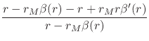
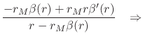
![]() , since that equation can be written as
, since that equation can be written as
![$\displaystyle \frac{r-r_{M}\left[r\beta'(r)\right]}{r-r_{M}\beta(r)}
\;\;\;\Rightarrow$](img275.png) |
|||
 |
|||
 |
|||
![$\displaystyle -\,
\frac{r_{M}}{2}\,
\frac
{\beta(r)-\left[r\beta'(r)\right]}
{r-r_{M}\beta(r)},$](img280.png) |
(55) |
where we again used our ansatz, as well as the solution for
![]() given
in Equation (54), and which therefore determines
given
in Equation (54), and which therefore determines ![]() in terms of
in terms of ![]() . Using now, once more, that result for
. Using now, once more, that result for
![]() and
the
and
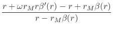
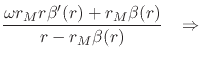
the ![]() component of the field equation, shown in
Equation (25), we can get the quantity
component of the field equation, shown in
Equation (25), we can get the quantity ![]() , since
that equation can be written as
, since
that equation can be written as
![$\displaystyle \frac
{r+\omega r_{M}\left[r\beta'(r)\right]}
{r-r_{M}\beta(r)}
\;\;\;\Rightarrow$](img284.png) |
|||
 |
|||
 |
|||
![$\displaystyle \frac{r_{M}}{2}\,
\frac
{\beta(r)+\omega\left[r\beta'(r)\right]}
{r-r_{M}\beta(r)},$](img289.png) |
(56) |
where we once again used our ansatz, and which therefore determines
![]() in terms of
in terms of ![]() . Note that
. Note that ![]() is not equal
to
is not equal
to ![]() , as would be the case for the Schwarzschild solution.
However, it is to be expected that
, as would be the case for the Schwarzschild solution.
However, it is to be expected that ![]() has
has ![]() as its
as its
![]() asymptotic limit. With this we have two of the three
quantities that appear in the left-hand side of the
asymptotic limit. With this we have two of the three
quantities that appear in the left-hand side of the ![]() component of
the field equation, shown in Equation (26). Since we have
that
component of
the field equation, shown in Equation (26). Since we have
that
| (57) |
and using once again the result for
![]() given in
Equation (54), the
given in
Equation (54), the ![]() component equation given in
Equation (26) can now be written in the form
component equation given in
Equation (26) can now be written in the form
In order to be able to write out this equation, we must now calculate in
terms of ![]() the quantity
the quantity
![]() . We can do this
by simply differentiating the quantity
. We can do this
by simply differentiating the quantity
![]() . The
detailed calculation can be found in Subsection A.2.1 of
Appendix A, and the result is
. The
detailed calculation can be found in Subsection A.2.1 of
Appendix A, and the result is
![\begin{displaymath}
r\left[r\nu'(r)\right]'
=
r_{M}\,
\frac
{
\left(
\beg...
...r
\beta(r)
\end{array} \right)
}
{2[r-r_{M}\beta(r)]^{2}},
\end{displaymath}](img295.png) |
(59) |
which therefore determines ![]() in terms of
in terms of ![]() . We now have
all the quantities that appear in the left-hand side of the
. We now have
all the quantities that appear in the left-hand side of the ![]() component of the field equation, shown in Equation (26). In
fact, just as in the case of the vacuum solution, the solution in the
presence of fluid matter is characterized by the following set of
quantities, this time written in terms of
component of the field equation, shown in Equation (26). In
fact, just as in the case of the vacuum solution, the solution in the
presence of fluid matter is characterized by the following set of
quantities, this time written in terms of ![]() ,
,
Note that the quantity ![]() remains undetermined, which does
not really present a problem, since it does not appear in the components
of the field equation. Once
remains undetermined, which does
not really present a problem, since it does not appear in the components
of the field equation. Once ![]() is determined in each particular
case,
is determined in each particular
case, ![]() can be obtained from
can be obtained from ![]() by straightforward
integration. These expressions are to be used in what follows in order to
define the asymptotic conditions in the
by straightforward
integration. These expressions are to be used in what follows in order to
define the asymptotic conditions in the ![]() asymptotic limit.
This is what we will do next. Later on we will return to the discussion of
the single equation yet to be satisfied, the
asymptotic limit.
This is what we will do next. Later on we will return to the discussion of
the single equation yet to be satisfied, the ![]() component equation
in the form shown in Equation (58).
component equation
in the form shown in Equation (58).
On the one hand, in Section 3 we calculated from the vacuum
solution the values of the ![]() asymptotic limits, for the various
corresponding quantities involved in the solution in the presence of fluid
mater, asymptotic values that were given in
Equations (47)--(51). On the other hand, in
this section we calculated the solution in the presence of fluid matter,
and listed what is essentially the same set of relevant quantities in
Equations (60)--(64). We are now ready to
discuss the corresponding asymptotic conditions. It is to be expected, of
course, that they will result in corresponding asymptotic conditions on
asymptotic limits, for the various
corresponding quantities involved in the solution in the presence of fluid
mater, asymptotic values that were given in
Equations (47)--(51). On the other hand, in
this section we calculated the solution in the presence of fluid matter,
and listed what is essentially the same set of relevant quantities in
Equations (60)--(64). We are now ready to
discuss the corresponding asymptotic conditions. It is to be expected, of
course, that they will result in corresponding asymptotic conditions on
![]() and its derivatives. We start by discussing the asymptotic
condition on
and its derivatives. We start by discussing the asymptotic
condition on ![]() . As we already discussed before, the expression
in Equation (48) can only be the asymptotic limit of the
expression in Equation (61) if we have that
. As we already discussed before, the expression
in Equation (48) can only be the asymptotic limit of the
expression in Equation (61) if we have that
| (65) |
Note that we do not have to worry directly about the asymptotic condition
on ![]() , because
, because ![]() itself does not appear in the component
equations, which contain only its derivatives. Therefore, next we discuss
the asymptotic condition on
itself does not appear in the component
equations, which contain only its derivatives. Therefore, next we discuss
the asymptotic condition on ![]() . Given that
. Given that ![]() , the
expression in Equation (50) can only be the asymptotic limit
of the expression in Equation (63) if we have that
, the
expression in Equation (50) can only be the asymptotic limit
of the expression in Equation (63) if we have that
| (66) |
Next we discuss the asymptotic condition on ![]() . It is quite clear
that the conditions above on
. It is quite clear
that the conditions above on ![]() and
and ![]() are sufficient to
ensure that the expression in Equation (49) will be the
asymptotic limit of the expression in Equation (62). Let us
recall that, once we have
are sufficient to
ensure that the expression in Equation (49) will be the
asymptotic limit of the expression in Equation (62). Let us
recall that, once we have ![]() in terms of a known function
in terms of a known function
![]() , we can obtain
, we can obtain ![]() from
from ![]() by straightforward
integration. When doing this integration, the integration constant must be
chosen so that
by straightforward
integration. When doing this integration, the integration constant must be
chosen so that ![]() , just like
, just like ![]() , goes to zero for
, goes to zero for
![]() , of course. In that limit we also expect that
, of course. In that limit we also expect that
![]() . Finally, we discuss the asymptotic condition on
. Finally, we discuss the asymptotic condition on
![]() . Given that
. Given that ![]() and that
and that
![]() , the expression in
Equation (51) can only be the asymptotic limit of the
expression in Equation (64) if we have that
, the expression in
Equation (51) can only be the asymptotic limit of the
expression in Equation (64) if we have that
| (67) |
Therefore, we have the complete set of asymptotic conditions to be
satisfied by ![]() and its derivatives,
and its derivatives,
| (68) |
We must now discuss what happens near ![]() . At this point we will have
conditions associated to the regularity of the energy density. If we
consider that, according to the definitions in Section 2, the
energy density is given by
. At this point we will have
conditions associated to the regularity of the energy density. If we
consider that, according to the definitions in Section 2, the
energy density is given by
| (69) |
where we also have that
![]() , as shown in
Equation (54), it follows that we have
, as shown in
Equation (54), it follows that we have
| (70) |
If the energy density ![]() is to be non-singular at
is to be non-singular at ![]() , and have
a limited integral around that point, then we must have that the limit
, and have
a limited integral around that point, then we must have that the limit
| (71) |
exists and is finite. This implies that at least for the first derivative
of ![]() we must have that
we must have that ![]() . In fact, since we must also
have that
. In fact, since we must also
have that
![]() when
when ![]() , one can show that the same has
to be true for the second derivative as well, that is, we also have that
, one can show that the same has
to be true for the second derivative as well, that is, we also have that
![]() . This leads us to a picture of a function
. This leads us to a picture of a function ![]() that
has both zero derivative and zero second derivative at both ends of the
real
that
has both zero derivative and zero second derivative at both ends of the
real ![]() semi-axis.
semi-axis.
One may also argue that it is necessary that ![]() not be a
strictly positive number. The argument leading to this condition is as
follows. According to the motivation leading to the construction of our
solution, the quantity
not be a
strictly positive number. The argument leading to this condition is as
follows. According to the motivation leading to the construction of our
solution, the quantity ![]() , where
, where
![]() and
and
![]() , is effectively a certain fraction of the total mass
, is effectively a certain fraction of the total mass
![]() . If
. If ![]() then this quantity has a finite and non-zero positive
limit when we make
then this quantity has a finite and non-zero positive
limit when we make ![]() . What this means is that there is a certain
finite and non-zero mass, given by
. What this means is that there is a certain
finite and non-zero mass, given by ![]() , which is inside a
sphere whose surface is at the radial position
, which is inside a
sphere whose surface is at the radial position ![]() , and that this holds
for all
, and that this holds
for all ![]() . However, this means that for some value of
. However, this means that for some value of ![]() this
finite and non-zero mass will be inside the Schwarzschild radius
associated to itself, thus leading to the existence of an event horizon
within the matter distribution, which contradicts our hypotheses here. In
order to avoid this, and assuming that
this
finite and non-zero mass will be inside the Schwarzschild radius
associated to itself, thus leading to the existence of an event horizon
within the matter distribution, which contradicts our hypotheses here. In
order to avoid this, and assuming that
![]() , we might
be tempted to conclude that we must have that
, we might
be tempted to conclude that we must have that
| (72) |
that is, that we must have ![]() . However, we should not take this
heuristic motivation too seriously, and while it seems inevitably true
that we cannot have
. However, we should not take this
heuristic motivation too seriously, and while it seems inevitably true
that we cannot have ![]() , we also cannot definitely assert
that we must have
, we also cannot definitely assert
that we must have ![]() , because there is really no reason why
, because there is really no reason why
![]() cannot be negative. Instead, once the ansatz given in
Equation (53) is assumed, we must then follow wherever the
field equation takes us. In fact, contrary to what the heuristic intuition
may seem to indicate,
cannot be negative. Instead, once the ansatz given in
Equation (53) is assumed, we must then follow wherever the
field equation takes us. In fact, contrary to what the heuristic intuition
may seem to indicate, ![]() is indeed always negative. When
is indeed always negative. When
![]() becomes negative it becomes impossible for the factor
becomes negative it becomes impossible for the factor
![]() to diverge, as it does at the event horizon of the
Schwarzschild solution, and this makes the solution regular and avoids the
existence of event horizons within the matter distribution. Considering
the fact that, due to the positivity of the energy, we must have
to diverge, as it does at the event horizon of the
Schwarzschild solution, and this makes the solution regular and avoids the
existence of event horizons within the matter distribution. Considering
the fact that, due to the positivity of the energy, we must have
![]() for all
for all ![]() , and taking into account the asymptotic
conditions derived here for
, and taking into account the asymptotic
conditions derived here for ![]() and its derivatives, as well as the
conditions at
and its derivatives, as well as the
conditions at ![]() , we can state that the function
, we can state that the function ![]() must have a
very simple qualitative behavior, going monotonically from some negative
value at
must have a
very simple qualitative behavior, going monotonically from some negative
value at ![]() to the value
to the value ![]() for
for ![]() . We have therefore the
complete set of relevant conditions at the two ends of the real
. We have therefore the
complete set of relevant conditions at the two ends of the real ![]() semi-axis,
semi-axis,
| (73) |
Note that, since we have here a second-order field equation, which will
give origin to a second-order equation for ![]() , we in fact can
satisfy only two independent conditions using the corresponding
integration constants. Therefore any additional conditions must arise as
automatic consequences of the first two. As we will see, it is possible to
reduce the equation for
, we in fact can
satisfy only two independent conditions using the corresponding
integration constants. Therefore any additional conditions must arise as
automatic consequences of the first two. As we will see, it is possible to
reduce the equation for ![]() to a form in which one has only two
free parameters to deal with, both physically meaningful, one of which
will be given by the total mass
to a form in which one has only two
free parameters to deal with, both physically meaningful, one of which
will be given by the total mass ![]() present, leading to the parameter
present, leading to the parameter
![]() , and only one, the parameter
, and only one, the parameter ![]() , which directly affects the
integration process itself. Since we have fewer parameters to adjust than
conditions to meet, the problem can only be solved if there are internal
consistency structures within the system that guarantee that most
conditions are automatically met when we adjust the parameters in order to
satisfy what conditions we can. We will see that this is indeed the case.
, which directly affects the
integration process itself. Since we have fewer parameters to adjust than
conditions to meet, the problem can only be solved if there are internal
consistency structures within the system that guarantee that most
conditions are automatically met when we adjust the parameters in order to
satisfy what conditions we can. We will see that this is indeed the case.
![$\displaystyle \left[
r\,{\rm e}^{-2\lambda(r)}
\right]'$](img188.png)

![\begin{displaymath}
r\left[r\nu'(r)\right]'(r)
=
\frac{r_{M}}{2}\,
\frac
{
...
... r
\beta(r)
\end{array} \right)
}
{[r-r_{M}\beta(r)]^{2}}.
\end{displaymath}](img297.png)