Next: Solution in Vacuum Up: Extension of the Schwarzschild Previous: Introduction
Here we will review the main points and equations relating to the Einstein
field equations under the set of symmetry conditions that we are to impose
on them. Our initial development here will follow closely the one
presented in [#!DiracGravity!#]. Under the conditions of time
independence and of spherical symmetry around the origin of a spherical
system of coordinates
![]() , the Schwarzschild system of
coordinates, the most general possible metric is given by the invariant
interval, written in terms of this spherical system of coordinates,
, the Schwarzschild system of
coordinates, the most general possible metric is given by the invariant
interval, written in terms of this spherical system of coordinates,
| (1) |
where ![]() and
and ![]() are two functions of only
are two functions of only ![]() . As one can
see, in this work we will use the time-like signature
. As one can
see, in this work we will use the time-like signature ![]() ,
following [#!DiracGravity!#]. Expressing the coefficients of
,
following [#!DiracGravity!#]. Expressing the coefficients of ![]() and
and
![]() by the exponentials shown ensures that they have the physically
required signs.
by the exponentials shown ensures that they have the physically
required signs.
Let us now comment on the physical interpretation of these coordinates. In
this coordinate system ![]() is such that a sphere centered at the origin
is such that a sphere centered at the origin
![]() and with its surface located at the position
and with its surface located at the position ![]() has total physical
surface area equal to
has total physical
surface area equal to ![]() . However,
. However, ![]() is not the true
physical distance from the surface of the sphere to the origin, and
furthermore
is not the true
physical distance from the surface of the sphere to the origin, and
furthermore ![]() is not a variation of physical length in the radial
direction. Note also that the time variable
is not a variation of physical length in the radial
direction. Note also that the time variable ![]() is not the true
proper time at each spatial position. These two coordinates only recover
their usual meanings in the
is not the true
proper time at each spatial position. These two coordinates only recover
their usual meanings in the ![]() asymptotic limit, if that limit
is accessible. In general the element of physical length in the radial
direction is given by
asymptotic limit, if that limit
is accessible. In general the element of physical length in the radial
direction is given by
![]() , and the element of proper time
at each position is given by
, and the element of proper time
at each position is given by
![]() . Finally note that, on the
other hand, the quantities
. Finally note that, on the
other hand, the quantities ![]() and
and
![]() are in fact
true physical elements of arc length on the surface of the sphere, that
is, on the spherical surface located at the position
are in fact
true physical elements of arc length on the surface of the sphere, that
is, on the spherical surface located at the position ![]() .
.
From this invariant interval we can simply read out the metric tensor
![]() , that is, the metric tensor in its covariant form,
, that is, the metric tensor in its covariant form,
![\begin{displaymath}
g_{\mu\nu}
=
\left[
\rule{0em}{8ex}
\begin{array}{llll}...
...0 \hspace{4em} &
-r^{2}\sin^{2}(\theta)
\end{array} \right].
\end{displaymath}](img46.png) |
(2) |
Note that we have for the determinant
![]() of the matrix
of the matrix
![]() the value
the value
| (3) |
which is not zero for ![]() except at the two poles
except at the two poles ![]() and
and
![]() , which are just the usual singularities of the spherical
system of coordinates, and can therefore be safely ignored. Recalling that
, which are just the usual singularities of the spherical
system of coordinates, and can therefore be safely ignored. Recalling that
![]() is the identity matrix, we obtain at
once the metric tensor
is the identity matrix, we obtain at
once the metric tensor ![]() , that is, the metric tensor in its
contravariant form, which is the inverse matrix to the diagonal matrix
, that is, the metric tensor in its
contravariant form, which is the inverse matrix to the diagonal matrix
![]() given above. The matrix
given above. The matrix ![]() in invertible almost
everywhere due to the fact that
in invertible almost
everywhere due to the fact that ![]() almost everywhere, and the
inverse is immediately found to be given by
almost everywhere, and the
inverse is immediately found to be given by
![\begin{displaymath}
g^{\mu\nu}
=
\left[
\rule{0em}{8ex}
\begin{array}{llll}...
...\hspace{5em} &
-r^{-2}\sin^{-2}(\theta)
\end{array} \right].
\end{displaymath}](img55.png) |
(4) |
The next step in the geometric development is to calculate from
![]() and
and ![]() the Christoffel symbol of the second kind
the Christoffel symbol of the second kind
![]() , which gives us the metric-compatible and
torsion-free connection for the pseudo-Riemannian parallel transport in
spacetime. It is given in terms of the metric tensor by
, which gives us the metric-compatible and
torsion-free connection for the pseudo-Riemannian parallel transport in
spacetime. It is given in terms of the metric tensor by
 |
(5) |
This is the Christoffel symbol of the second kind, while the same quantity
with all indices downstairs is the Christoffel symbol of the first kind.
They are symmetric on the last two indices, as one can see, and they are
non-tensors, because the derivative of a second-rank tensor is not a
tensor. Note that the three terms within parenthesis correspond to cyclic
permutations of the three indices. From now on the derivatives with
respect to ![]() of
of ![]() ,
, ![]() , and any other quantities that
depend only on
, and any other quantities that
depend only on ![]() , will be denoted by primes.
, will be denoted by primes.
In this calculation many of the components of
![]() turn out to be zero, as reported
in [#!DiracGravity!#], and if one recalls that this quantity is symmetric
on the pair of indices
turn out to be zero, as reported
in [#!DiracGravity!#], and if one recalls that this quantity is symmetric
on the pair of indices ![]() , one gets the results, written in
matrix form on the two lower indices, that are shown in
Table 1. This matrix form is very useful as a basis for further
calculations, such as that of the curvature tensor. Using these
expressions in the equation defining the Ricci curvature tensor
, one gets the results, written in
matrix form on the two lower indices, that are shown in
Table 1. This matrix form is very useful as a basis for further
calculations, such as that of the curvature tensor. Using these
expressions in the equation defining the Ricci curvature tensor
![]() in terms of the connection, which is given by
in terms of the connection, which is given by
| (6) |
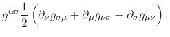
one gets a diagonal matrix for this curvature tensor, in its covariant form,
![\begin{displaymath}
R_{\mu\nu}
=
\left[
\rule{0em}{8ex}
\begin{array}{llll}...
...\hspace{2em} &
0 \hspace{2em} &
R_{33}
\end{array} \right],
\end{displaymath}](img65.png) |
(7) |
with the four diagonal elements given in [#!DiracGravity!#], which are
![$\displaystyle \left\{
-
\nu''(r)
+
\lambda'(r)\nu'(r)
-
\left[
\nu'(r)
\right]^{2}
-
\frac{2\nu'(r)}{r}
\right\}
\,{\rm e}^{2\nu(r)-2\lambda(r)},$](img67.png) |
|||
![$\displaystyle \left\{
\nu''(r)
-
\lambda'(r)\nu'(r)
+
\left[
\nu'(r)
\right]^{2}
-
\frac{2\lambda'(r)}{r}
\right\},$](img69.png) |
|||
| (8) |
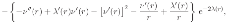
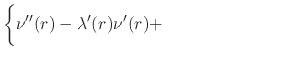
With the use of ![]() the same quantities can be written, in mixed
form, as
the same quantities can be written, in mixed
form, as
![$\displaystyle \left\{
-
\nu''(r)
+
\lambda'(r)\nu'(r)
-
\left[
\nu'(r)
\right]^{2}
-
\frac{2\nu'(r)}{r}
\right\}
\,{\rm e}^{-2\lambda(r)},$](img75.png) |
|||
![$\displaystyle \left\{
-
\nu''(r)
+
\lambda'(r)\nu'(r)
-
\left[
\nu'(r)
\right]^{2}
+
\frac{2\lambda'(r)}{r}
\right\}
\,{\rm e}^{-2\lambda(r)},$](img77.png) |
|||
![$\displaystyle -
\left[
\frac{1}{r^{2}}
+
\frac{\nu'(r)}{r}
-
\frac{\lambda'(r)}{r}
\right]
\,{\rm e}^{-2\lambda(r)}
+
\frac{1}{r^{2}},$](img79.png) |
|||
![$\displaystyle -
\left[
\frac{1}{r^{2}}
+
\frac{\nu'(r)}{r}
-
\frac{\lambda'(r)}{r}
\right]
\,{\rm e}^{-2\lambda(r)}
+
\frac{1}{r^{2}}.$](img81.png) |
(9) |
We will tend to write all relevant tensor quantities in this mixed form,
which is the most useful for our purposes here. Note that the exponential
![]() has vanished from these expressions, which therefore
contain only the functions
has vanished from these expressions, which therefore
contain only the functions ![]() ,
, ![]() ,
, ![]() and
and
![]() . Note also that it turns out that
. Note also that it turns out that
![]() , as a
consequence of the symmetries that we imposed. The last geometric element
that we need to discuss here is the scalar curvature
, as a
consequence of the symmetries that we imposed. The last geometric element
that we need to discuss here is the scalar curvature
![]() ,
which can be written as
,
which can be written as
| (10) |
We therefore can write our result for the scalar curvature as
| (11) |
In the theory of General Relativity the equation determining the
gravitational field is written in terms of the Ricci curvature tensor
![]() . The equation also involves the matter energy-momentum tensor
. The equation also involves the matter energy-momentum tensor
![]() , which plays the role of the source of the gravitational
field. The Einstein gravitational field equation is a tensor equation
which, written in its mixed form, using our notation here, with the
signature
, which plays the role of the source of the gravitational
field. The Einstein gravitational field equation is a tensor equation
which, written in its mixed form, using our notation here, with the
signature ![]() , following [#!DiracGravity!#], is given by
, following [#!DiracGravity!#], is given by
| (12) |
where
![]() ,
, ![]() is the universal gravitational constant
and
is the universal gravitational constant
and ![]() is the speed of light.
is the speed of light.
Note that the imposition of spherical symmetry and time independence on
the solution of the Einstein field equation reduces the problem of finding
that solution to a much simpler one-dimensional one, on the variable ![]() .
While one can take any metric at all, so long as the functions involved in
it, such as
.
While one can take any metric at all, so long as the functions involved in
it, such as ![]() and
and ![]() , are differentiable to the second
order, and just calculate
, are differentiable to the second
order, and just calculate ![]() and
and ![]() in order to simply
verify whatever results for
in order to simply
verify whatever results for ![]() , with such a deeply non-linear
equation one is not free to choose the matter energy-momentum
tensor
, with such a deeply non-linear
equation one is not free to choose the matter energy-momentum
tensor ![]() in an arbitrary way. Both the general structure of
the theory and the symmetry conditions will impose restrictions on the
possible values of this tensor. For example, since we have, due to the
imposition of the symmetries, that
in an arbitrary way. Both the general structure of
the theory and the symmetry conditions will impose restrictions on the
possible values of this tensor. For example, since we have, due to the
imposition of the symmetries, that
![]() , and since we
also have that
, and since we
also have that
![]() , it follows at once that
, it follows at once that
![]() . Also, since
. Also, since ![]() and
and ![]() are
symmetric tensors, so must be
are
symmetric tensors, so must be ![]() .
.
At this point we must pause in order to consider what information we have
obtained so far about ![]() . First of all, since under the
current hypotheses the left-hand side of the Einstein field equation turns
out to be diagonal, and since we have also the additional fact that
the expressions of the last two component equations turn out to be
identical, the same must be true for the matter energy-momentum tensor
. First of all, since under the
current hypotheses the left-hand side of the Einstein field equation turns
out to be diagonal, and since we have also the additional fact that
the expressions of the last two component equations turn out to be
identical, the same must be true for the matter energy-momentum tensor
![]() on the right-hand side of the equation, which must
therefore be diagonal,
on the right-hand side of the equation, which must
therefore be diagonal,
and which must also satisfy
![]() . In addition to
this, since there are no dependencies on
. In addition to
this, since there are no dependencies on ![]() ,
, ![]() or
or ![]() , it
follows that
, it
follows that ![]() can depend only on
can depend only on ![]() . Note, however, that
we still do not have any further information about any possible
relations between
. Note, however, that
we still do not have any further information about any possible
relations between ![]() ,
, ![]() and
and ![]() . From
this point on, in order to simplify the notation, we will use the variable
names
. From
this point on, in order to simplify the notation, we will use the variable
names ![]() ,
, ![]() ,
, ![]() and
and ![]() for the diagonal
elements
for the diagonal
elements ![]() ,
, ![]() ,
, ![]() and
and
![]() , respectively, of the energy-momentum tensor
, respectively, of the energy-momentum tensor
![]() in its mixed form.
in its mixed form.
The main general consistency condition imposed by the structure of the
theory is that the covariant divergence of ![]() must vanish,
that is, the condition that we must have that
must vanish,
that is, the condition that we must have that
This is due to the fact that the combination of tensors that constitutes the left-hand side of the Einstein field equation satisfies the Bianci identity of the Ricci curvature tensor,
| (15) |
which therefore implies the requirement that the covariant divergence of
![]() must vanish,
must vanish,
| (16) |
Since ![]() and
and ![]() behave as constants under covariant
differentiation, we may then write this condition as the requirement on
behave as constants under covariant
differentiation, we may then write this condition as the requirement on
![]() given in Equation (14). At this point we must
calculate this consistency condition for the specific case of time
independence and spherical symmetry. In other words, we must now write
explicitly, under these conditions, the expression shown in
Equation (14). This rather long calculation is done in detail
in Section A.1 of Appendix A. As one can see there,
three of the four conditions in Equation (14) are
automatically satisfied, since it results from that calculation that
given in Equation (14). At this point we must
calculate this consistency condition for the specific case of time
independence and spherical symmetry. In other words, we must now write
explicitly, under these conditions, the expression shown in
Equation (14). This rather long calculation is done in detail
in Section A.1 of Appendix A. As one can see there,
three of the four conditions in Equation (14) are
automatically satisfied, since it results from that calculation that
| (17) |
Therefore, the only non-trivial condition is that given by
![]() , which results in
, which results in
| (18) |
and which can also be written as
Note that this consistency condition on
![]() ends up
involving only the element of the metric given by the function
ends up
involving only the element of the metric given by the function ![]() .
.
We now have at hand all the elements needed in order to write the Einstein
gravitational field equation under our hypotheses about the geometry, as
well as the relevant consistency condition. Using the elements
![]() and
and ![]() , as well as the fact that
, as well as the fact that
![]() , we may now write the left-hand side of
the components of the Einstein field equation, in mixed form, as
, we may now write the left-hand side of
the components of the Einstein field equation, in mixed form, as
 |
![$\displaystyle \left[
\frac{1}{r^{2}}
-
\frac{2\lambda'(r)}{r}
\right]
\,{\rm e}^{-2\lambda(r)}
-
\frac{1}{r^{2}},$](img128.png) |
||
 |
![$\displaystyle \left[
\frac{1}{r^{2}}
+
\frac{2\nu'(r)}{r}
\right]
\,{\rm e}^{-2\lambda(r)}
-
\frac{1}{r^{2}},$](img130.png) |
||
 |
 |
||
 |
 |
(20) |
It thus results that we get some fairly simple expressions for the
left-hand sides of the four components of the field equation in mixed
form. Note once more that the exponential ![]() is absent from
these expressions, and also that the expressions of the last two component
equations are identical, and therefore not independent from each other. We
must now write the right-hand side of these equations, and thus introduce
the energy-momentum tensor
is absent from
these expressions, and also that the expressions of the last two component
equations are identical, and therefore not independent from each other. We
must now write the right-hand side of these equations, and thus introduce
the energy-momentum tensor
![]() that was discussed before.
that was discussed before.
Let us recall that, for an homogeneous and isotropic cosmological
spacetime, containing equally homogeneous and isotropic fluid matter, in
the co-moving system of coordinates, in which the matter is locally at
rest, we would have that
![]() , where
, where ![]() is the energy
density, and that
is the energy
density, and that
![]() , where
, where ![]() is the
pressure. We can expect a similar situation in our case here, for the
values of the components of the energy-momentum tensor. Note that the pure radiation condition given by the equation of state
is the
pressure. We can expect a similar situation in our case here, for the
values of the components of the energy-momentum tensor. Note that the pure radiation condition given by the equation of state ![]() translates here to the simple invariant condition
translates here to the simple invariant condition ![]() on the
trace of
on the
trace of
![]() . Note also that this condition holds for any
type of massless matter field. It is important to observe that up to this
point we have assumed no more about these quantities than what is implied
by the structure of the field equation itself. Since we must have that
. Note also that this condition holds for any
type of massless matter field. It is important to observe that up to this
point we have assumed no more about these quantities than what is implied
by the structure of the field equation itself. Since we must have that
![]() as a consequence of the symmetries that we imposed, we
have only three independent components of the field equation, to which we
now add the consistency condition as an ancillary condition,
as a consequence of the symmetries that we imposed, we
have only three independent components of the field equation, to which we
now add the consistency condition as an ancillary condition,
![$\displaystyle \left[
\frac{1}{r^{2}}
-
\frac{2\lambda'(r)}{r}
\right]
\,{\rm e}^{-2\lambda(r)}
-
\frac{1}{r^{2}}$](img142.png) |
|||
![$\displaystyle \left[
\frac{1}{r^{2}}
+
\frac{2\nu'(r)}{r}
\right]
\,{\rm e}^{-2\lambda(r)}
-
\frac{1}{r^{2}}$](img144.png) |
|||
 |
|||
![$\displaystyle \left.
+
\left[
\nu'(r)
\right]^{2}
+
\frac{\nu'(r)}{r}
-
\frac{\lambda'(r)}{r}
\rule{0em}{3ex}
\right\}
\,{\rm e}^{-2\lambda(r)}$](img147.png) |
where we recall that
![]() . We will now impose on the
components of
. We will now impose on the
components of
![]() the equation of state for fluid matter.
Since the equation of state determines the nature of the fluid, and
assuming that no phase transitions occur within the volume occupied by the
matter, we must have the same equation of state throughout the volume of
the fluid matter. In other words, the equation of state must not dependent
on the position
the equation of state for fluid matter.
Since the equation of state determines the nature of the fluid, and
assuming that no phase transitions occur within the volume occupied by the
matter, we must have the same equation of state throughout the volume of
the fluid matter. In other words, the equation of state must not dependent
on the position ![]() . Both the energy density
. Both the energy density ![]() and the pressure
and the pressure
![]() may depend on
may depend on ![]() , but the relations between them may not. This
means that we are assuming, in this simplest case, that there is a certain
homogeneity regarding the state of the matter, which is assumed not
to undergo a phase transition along the possible values of
, but the relations between them may not. This
means that we are assuming, in this simplest case, that there is a certain
homogeneity regarding the state of the matter, which is assumed not
to undergo a phase transition along the possible values of ![]() . This
implies that we should have the relations
. This
implies that we should have the relations
| (22) |
which automatically satisfy the condition that
![]() , and
where
, and
where ![]() is a positive real number in the interval
is a positive real number in the interval ![]() . The
value
. The
value ![]() corresponds to pressureless dust and the value
corresponds to pressureless dust and the value
![]() corresponds to pure relativistic radiation. The value of
corresponds to pure relativistic radiation. The value of
![]() in this range determines what fraction of the energy is bound in
the form or rest mass and what fraction is in the form of relativistic
radiation. Multiplying the first three component equations in
Equation (21) by
in this range determines what fraction of the energy is bound in
the form or rest mass and what fraction is in the form of relativistic
radiation. Multiplying the first three component equations in
Equation (21) by ![]() and making the replacements
indicated above, which result in the fluid matter being described by the
single function
and making the replacements
indicated above, which result in the fluid matter being described by the
single function ![]() , we get
, we get
![$\displaystyle \left\{
\rule{0em}{3ex}
r^{2}\nu''(r)
-
\left[
r\lambda'(r)
\right]
\left[
r\nu'(r)
\right]
+
\right.
\hspace{6em}$](img162.png) |
|||
![$\displaystyle \left.
+
\left[
r\nu'(r)
\right]^{2}
+
\left[
r\nu'(r)
\right]
-
\left[
r\lambda'(r)
\right]
\rule{0em}{3ex}
\right\}
\,{\rm e}^{-2\lambda(r)}$](img163.png) |
| (23) |
At this point it is convenient to write all the equations in terms of the
single function given by
![]() , which also happens
to be dimensionless, because due to the dimensions of the Einstein field
equation the quantity
, which also happens
to be dimensionless, because due to the dimensions of the Einstein field
equation the quantity
![]() has the dimensions of
has the dimensions of
![]() ,
,
These are the four equations that must be satisfied by the functions
![]() ,
, ![]() and
and
![]() that represent a solution of the
Einstein gravitational field equation in the presence of fluid matter,
under the hypotheses of time independence, spherical symmetry and a simple
homogeneous local equation of state for the fluid matter. In the sequence
we will first recover the solution for empty space, that is, we will
derive from these equations the Schwarzschild solution, and then we will
establish the solution in the presence of the fluid matter. Ultimately,
the Schwarzschild solution will play the role of being the
that represent a solution of the
Einstein gravitational field equation in the presence of fluid matter,
under the hypotheses of time independence, spherical symmetry and a simple
homogeneous local equation of state for the fluid matter. In the sequence
we will first recover the solution for empty space, that is, we will
derive from these equations the Schwarzschild solution, and then we will
establish the solution in the presence of the fluid matter. Ultimately,
the Schwarzschild solution will play the role of being the ![]() asymptotic limit of the solution in the presence of localized fluid
matter.
asymptotic limit of the solution in the presence of localized fluid
matter.
![\begin{table}\centering
\begin{eqnarray*}
\Gamma^{0}_{\;\;\mu\nu}
& = &
\lef...
...cot(\theta) &
0 \hspace{3em}
\end{array} \right].
\end{eqnarray*} \end{table}](img61.png)
![\begin{displaymath}
T_{\mu}^{\nu}
=
\left[
\rule{0em}{8ex}
\begin{array}{ll...
...e{2em} &
0 \hspace{2em} &
T_{3}^{3}(r)
\end{array} \right],
\end{displaymath}](img101.png)