Next: Analytical Character of the Up: On the Convergence of Previous: Extension of the Result
The complex arithmetic used in the demonstration of the theorem can be
used, not only to prove the convergence of the series, but also as an
algorithm to accomplish an efficient numerical evaluation of the limit of
the series. This can be very useful, because series ![]() of the
type examined here may converge extremely slowly. Let us recall that we
have for the partial sums of the series
of the
type examined here may converge extremely slowly. Let us recall that we
have for the partial sums of the series
![]()
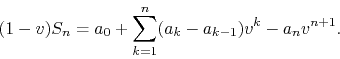
By our hypotheses, in the ![]() limit the last term vanishes, and
therefore we may write for the series
limit the last term vanishes, and
therefore we may write for the series
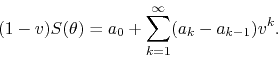
Observe that all the terms in the sum in the right-hand side are negative,
due to the fact that the coefficients decrease monotonically. Unlike the
original series for ![]() , the series in the right-hand side in this
formula is always absolutely convergent, as we saw during the proof of the
theorem. This series converges therefore much faster than the original
one, when that original one is not absolutely convergent. We may define
new symbols
, the series in the right-hand side in this
formula is always absolutely convergent, as we saw during the proof of the
theorem. This series converges therefore much faster than the original
one, when that original one is not absolutely convergent. We may define
new symbols ![]() for its coefficients,
for its coefficients,
while for ![]() we adopt the definition
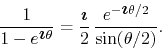
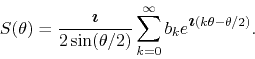
we adopt the definition ![]() , in terms of which
we may write that
, in terms of which
we may write that
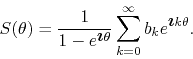
which holds so long as ![]() . In order to identify the real and
imaginary parts of this expression, which are related respectively to the
series of cosines and the series of sines, we write it back in terms of
. In order to identify the real and
imaginary parts of this expression, which are related respectively to the
series of cosines and the series of sines, we write it back in terms of
![]() , obtaining
, obtaining
The first factor in the right-hand side can be written as
If we substitute this in the expression for the series, we get
From this we may easily identify the series of sines and of cosines, and in this way we obtain for them the relations
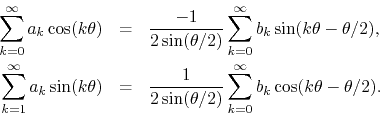
Separating once again the ![]() terms, we get
terms, we get
![\begin{eqnarray*}
\sum_{k=0}^{\infty}a_{k}\cos(k\theta)
& = &
\frac{a_{0}}{2}...
...}{2\sin(\theta/2)}
\sum_{k=1}^{\infty}b_{k}\cos[(k-1/2)\theta].
\end{eqnarray*}](img170.png)
The initial terms of these two series can be recognized as the coordinates
![]() and
and ![]() of the initial center of rotation. Note that the
other terms in the right-hand sides have half-integers in their arguments,
rather than the usual integers of the Fourier series. They may be
interpreted as well as series over only odd indices
of the initial center of rotation. Note that the
other terms in the right-hand sides have half-integers in their arguments,
rather than the usual integers of the Fourier series. They may be
interpreted as well as series over only odd indices ![]() , with the
half-angle
, with the
half-angle ![]() as argument.
as argument.
For coefficients ![]() that satisfy the hypotheses of our theorem and
that approach zero too slowly for the original series to be absolutely
convergent, the series in the right-hand sides converge much faster than
the corresponding ones in the left-hand sides, and therefore can be used
to calculate approximations to the same limits in a much more efficient
way when
that satisfy the hypotheses of our theorem and
that approach zero too slowly for the original series to be absolutely
convergent, the series in the right-hand sides converge much faster than
the corresponding ones in the left-hand sides, and therefore can be used
to calculate approximations to the same limits in a much more efficient
way when ![]() . This constitutes therefore a numerical technique for
the calculations of these limits. By using this technique one approaches
the limit by following the drift of the center
. This constitutes therefore a numerical technique for
the calculations of these limits. By using this technique one approaches
the limit by following the drift of the center ![]() , rather than
the propagation of the chain of the original series
, rather than
the propagation of the chain of the original series ![]() . In
general, even if the coefficients
. In
general, even if the coefficients ![]() do not satisfy our hypothesis of
monotonicity, whenever the series
do not satisfy our hypothesis of
monotonicity, whenever the series

converges, so does the original series ![]() , so long as
, so long as ![]() tends to zero as
tends to zero as ![]() . Hence, this numerical technique may be
useful even in cases when not all our hypotheses are satisfied.
. Hence, this numerical technique may be
useful even in cases when not all our hypotheses are satisfied.
Each one of the extensions of the theorem to other cases, which were
discusses previously, also comes with corresponding summation formulas
similar to the ones presented above, which in each case may be used for
the efficient numerical estimation of the limits. For example, we saw that
the result can be extended to series with non-zero coefficients only for
even ![]() , that is for
, that is for ![]() , and if we consider the angle
, and if we consider the angle
![]() we may write such a series as
we may write such a series as
which has exactly the same structure as the series just discussed, so that
we may write at once that, for
![]() for all integers
for all integers ![]() ,
,
![\begin{eqnarray*}
\sum_{j=0}^{\infty}a_{j}\cos(j\theta')
& = &
\frac{a_{0}}{2...
...2\sin(\theta'/2)}
\sum_{j=1}^{\infty}b_{j}\cos[(j-1/2)\theta'],
\end{eqnarray*}](img178.png)
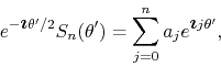
where
![]() , for
, for
![]() , and where once more
the two initial terms are the coordinates
, and where once more
the two initial terms are the coordinates ![]() and
and ![]() of the
initial center of rotation. Writing directly in terms of
of the
initial center of rotation. Writing directly in terms of ![]() we have
we have
![\begin{eqnarray*}
\sum_{j=0}^{\infty}a_{j}\cos(2j\theta)
& = &
\frac{a_{0}}{2...
...c{1}{2\sin(\theta)}
\sum_{j=1}^{\infty}b_{j}\cos[(2j-1)\theta],
\end{eqnarray*}](img181.png)
where we have now the condition that
![]() for all integers
for all integers
![]() . Note that in this case, while the series on the left are Fourier
series over only the even indices, the ones on the right are over only odd
indices. The case in which the series has non-zero coefficients only for
odd
. Note that in this case, while the series on the left are Fourier
series over only the even indices, the ones on the right are over only odd
indices. The case in which the series has non-zero coefficients only for
odd ![]() , that is for
, that is for ![]() , can be treated in a similar way. As we saw
before, in this case we may write the series as
, can be treated in a similar way. As we saw
before, in this case we may write the series as
which once more has the same structure as before, except for the
additional overall exponential factor. We get therefore in this case, for
the series written in terms of ![]() ,
,
which then leads to
![\begin{eqnarray*}
\sum_{j=0}^{\infty}a_{j}\cos[(j+1/2)\theta']
& = &
0
-
\f...
...ac{1}{2\sin(\theta'/2)}
\sum_{j=1}^{\infty}b_{j}\cos(j\theta'),
\end{eqnarray*}](img186.png)
where
![]() , for
, for
![]() , and where we see
that the two coordinates of the initial center of rotation are now
, and where we see
that the two coordinates of the initial center of rotation are now ![]() and
and
![]() . Writing directly in terms of
. Writing directly in terms of ![]() we have
we have
![\begin{eqnarray*}
\sum_{j=0}^{\infty}a_{j}\cos[(2j+1)\theta]
& = &
-\,\frac{1...
...\frac{1}{2\sin(\theta)}
\sum_{j=1}^{\infty}b_{j}\cos(2j\theta),
\end{eqnarray*}](img189.png)
where we have the same condition that
![]() for all integers
for all integers
![]() . Note that in this case, while the series on the left are Fourier
series over only the odd indices, the ones on the right are over only even
indices.
. Note that in this case, while the series on the left are Fourier
series over only the odd indices, the ones on the right are over only even
indices.