Next: Heat Conduction in a Up: Appendix: Examples of Use Previous: The Plucked String
Consider an empty two-dimensional rectangular box with electrically conducting walls kept at given values of the electric potential, as shown on Figure 3. The electrostatic potential within the box is given by Laplace's equation,
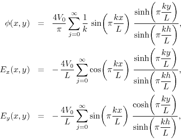
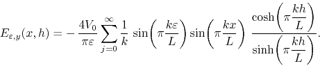
The boundary values are as shown in the illustration. Note that, as indicated in the figure, the top surface cannot be considered as being in electric contact with the other ones, if the potentials are to be kept as shown. However, in the resolution of the problem this fact is not taken explicitly into account. The solution of the problem can be given in terms of mixed Fourier and hyperbolic series for the electric potential and for the two Cartesian components of the electric field, which is obtained as minus the gradient of the potential,
 |
where ![]() . Note that so long as
. Note that so long as ![]() all these series are absolutely
convergent and uniformly convergent along the direction
all these series are absolutely
convergent and uniformly convergent along the direction ![]() . In fact, in
this case they converge to
. In fact, in
this case they converge to ![]() functions of
functions of ![]() . This is so
because the ratios of hyperbolic functions decrease to zero exponentially
fast with
. This is so
because the ratios of hyperbolic functions decrease to zero exponentially
fast with ![]() when
when ![]() . However, for
. However, for ![]() , that is at the top surface,
these factors cease to approach zero as
, that is at the top surface,
these factors cease to approach zero as ![]() , and then the
convergence status is much more precarious. The series for the potential
is still convergent, but not absolute or uniformly so. The series for the
field components diverge everywhere. This is caused by the neglect to take
into account the fact that the top surface must be electrically isolated
from the others, which causes the appearance of infinite electric fields
near the two top corners of the box. This is expressed as a singular
boundary condition at the top surface, with the form of a rectangular
pulse, discontinuous at
, and then the
convergence status is much more precarious. The series for the potential
is still convergent, but not absolute or uniformly so. The series for the
field components diverge everywhere. This is caused by the neglect to take
into account the fact that the top surface must be electrically isolated
from the others, which causes the appearance of infinite electric fields
near the two top corners of the box. This is expressed as a singular
boundary condition at the top surface, with the form of a rectangular
pulse, discontinuous at ![]() and
and ![]() , as shown in Figure 4.
, as shown in Figure 4.
One can change this by applying the first-order linear low-lass filter to
the boundary condition at the top surface, with a small range parameter
![]() , which has the effect of exchanging the discontinuities for
two very steep potential ramps, as is also shown in Figure 4.
Since the coefficients of the differential equation do not depend on
, which has the effect of exchanging the discontinuities for
two very steep potential ramps, as is also shown in Figure 4.
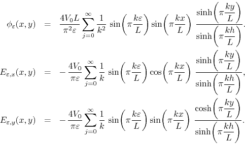
Since the coefficients of the differential equation do not depend on ![]() ,
we may at once write the solution for the filtered potential and for the
filtered electric field components, by simply plugging the filter factor
,
we may at once write the solution for the filtered potential and for the
filtered electric field components, by simply plugging the filter factor
![]() into the series,
into the series,
The series for the potential is now absolutely and uniformly convergent
everywhere within the box, including the top surface. The series for the
field components are still strongly convergent to ![]() functions
away from the top surface, and at that surface they are convergent almost
everywhere, although not absolutely or uniformly so. The solution changes
significantly only in the neighborhood of the two points were the original
singularity on the boundary conditions was located. If we write, as an
example, the field component
functions
away from the top surface, and at that surface they are convergent almost
everywhere, although not absolutely or uniformly so. The solution changes
significantly only in the neighborhood of the two points were the original
singularity on the boundary conditions was located. If we write, as an
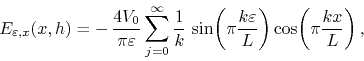
example, the field component
![]() at the top surface,
we get
at the top surface,
we get
where ![]() . One can show that this series is everywhere convergent
using trigonometric identities to write it in the form
. One can show that this series is everywhere convergent
using trigonometric identities to write it in the form
![\begin{displaymath}
E_{\varepsilon,x}(x,h)
=
\frac{2V_{0}}{\pi\varepsilon}
\...
...
-
\sin\!\left(\pi k\frac{x+\varepsilon}{L}\right)
\right].
\end{displaymath}](img214.png)
The two sine series obtained in this way have coefficients that converge
monotonically to zero and therefore are convergent by the Dirichlet test,
or alternatively by the monotonicity criterion discussed
in [3]. Therefore, the series for
![]() is
in fact everywhere convergent after the application of the filter. The
other field component at the top surface can be analyzed in a similar way.
It is given by
is
in fact everywhere convergent after the application of the filter. The
other field component at the top surface can be analyzed in a similar way.
It is given by
For large values of ![]() the ratio of hyperbolic functions tends to
the ratio of hyperbolic functions tends to ![]() .
In this case the analysis with the monotonicity criterion shown that the
series is convergent at all points except two, the points
.
In this case the analysis with the monotonicity criterion shown that the
series is convergent at all points except two, the points ![]() and
and
![]() . Further application of the first-order filter, or
the application of the second-order filter, can then be used to further
improve the situation.
. Further application of the first-order filter, or
the application of the second-order filter, can then be used to further
improve the situation.
We can say that the introduction of the filter in fact improved the
representation of the physical system in this problem, from the physical
standpoint, because the two steep potential ramps can be understood as a
representation of the electric potential within two thin slices of an
insulating material, of thickness ![]() , inserted between the top
surface and the two lateral ones. In fact, within a good dielectric this
is a very good representation of the electric potential. Once more we see
that the introduction of the filter brought the description of the
physical system closer to reality.
, inserted between the top
surface and the two lateral ones. In fact, within a good dielectric this
is a very good representation of the electric potential. Once more we see
that the introduction of the filter brought the description of the
physical system closer to reality.
The two remaining isolated points of divergence are in the field component normal to the surface, exactly at the point where we have the material interfaces between the conducting material of the upper wall and the insulating dielectric of the thin slices. This suggests that these remaining divergences are related to the imperfect representation of these material interfaces. In fact, the inclusion of the thin insulating slices introduces into the system two electric capacitors, and the divergences may be related to the known edge effects that occur at the edges of the plates of any capacitor, where electric charges tend to accumulate.
In this case the physical scale involved is that of the inter-material
transition at the interface, which may go right down to the molecular
level. Therefore it seems appropriate to use once more the first-order
filter on the boundary condition, this time with a range parameter
![]() . This will have the effect of smoothing out
the sharp transitions between the two materials. Regardless of the value
of the parameter
. This will have the effect of smoothing out
the sharp transitions between the two materials. Regardless of the value
of the parameter ![]() , this will render all the series
absolutely and uniformly convergent everywhere, since they will then all
have at least a factor of
, this will render all the series
absolutely and uniformly convergent everywhere, since they will then all
have at least a factor of ![]() in their coefficients.
in their coefficients.
The actual values of the field near the material interfaces will of course
depend on ![]() . If it turns out to be possible to measure these
field values well enough, it may be possible to determine an optimal value
of
. If it turns out to be possible to measure these
field values well enough, it may be possible to determine an optimal value
of ![]() based on experimental data, which will then establish a
rough model for the description of the material interface, from the
macroscopic point of view. We see therefore that this mathematical
technique may be turned into a tool for probing into aspects of the
structure of the physical world.
based on experimental data, which will then establish a
rough model for the description of the material interface, from the
macroscopic point of view. We see therefore that this mathematical
technique may be turned into a tool for probing into aspects of the
structure of the physical world.