The Plucked String

Consider the vibrating string of length $L$. In the small displacement approximation its movement is given by the wave equation

$$\frac{\partial^{2}f(x,t)}{\partial x^{2}} - \frac{1}{\nu^{2}}\, \frac{\partial^{2}f(x,t)}{\partial t^{2}} = 0,$$

where $\nu$ is the speed of the waves on the string and where $f(x,t)$ is the displacement from equilibrium at position $x$ and time $t$. The boundary conditions are $f(0,t)=0$ and $f(L,t)=0$ for all $t$. Let us suppose that the initial condition is that it is released from rest from the triangular position shown in Figure 2. Note that the initial position $f(x,0)$ is not differentiable at $x=L/2$. This is what we call the problem of the plucked string. The problem is to find $f(x,t)$ for all $x\in[0,L]$ and all $t\geq 0$. The solution of the problem can be given in terms of Fourier series for the position, velocity and acceleration of each point of the string,

$$\begin{eqnarray*} f(x,t) & = & \frac{8h}{\pi^{2}} \sum_{j=0}^{\infty} \frac... ...(\pi\frac{k\nu t}{L}\right) \sin\!\left(\pi\frac{kx}{L}\right), \end{eqnarray*}$$

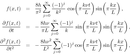
where $k=2j+1$. Note that the series for the position is absolutely and uniformly convergent. The series for the velocity can be shown to be everywhere convergent, but it is not absolutely or uniformly convergent. The series for the acceleration is simply everywhere divergent. In fact, in this case it can be shown that it represents two pulses with the form of Dirac delta ``functions'' going back and forth along the string and reflecting at its ends. This means that each point of the string is subjected to repeated impulsive accelerations. These are infinite accelerations that act for a single instant of time, producing however finite changes in the velocity. Obviously, we have here a rather singular situation.

Figure 2: Illustration of the original initial condition for the position of the plucked string, superposed with the filtered initial condition.

One can change this by applying the first-order linear low-lass filter to the initial condition, with a range parameter $\varepsilon$, which has the effect of exchanging the top of the triangle for an inverted arc of parabola that fits the two remaining segments in such a way that the resulting function is continuous and differentiable, as shown in Figure 2. Since the coefficients of the equation do not depend on $x$, we may obtain the filtered solution by simply plugging the filter factor $[\sin(\pi k\varepsilon/L)/(\pi k\varepsilon/L)]$ into the series, thus obtaining at once the filtered solution,

$$\begin{eqnarray*} f_{\varepsilon}(x,t) & = & \frac{8hL}{\pi^{3}\varepsilon} ... ...(\pi\frac{k\nu t}{L}\right) \sin\!\left(\pi\frac{kx}{L}\right). \end{eqnarray*}$$

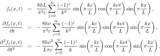
We see that now the series for the position and for the velocity are both absolutely and uniformly convergent. The series for the acceleration is now convergent, although it is still not absolutely or uniformly convergent. It now represents two rectangular pulses of width $\varepsilon$ propagating back and forth along the string and reflecting at its ends, with inversion of their sign. This means that each point of the string is now subjected repeatedly to a large but finite acceleration, proportional to $1/\varepsilon$, acting for a very short time, of the order of $\varepsilon/\nu$. One can show that the series for the acceleration is convergent using trigonometric identities to write it in the form

$$\begin{eqnarray*} \frac{\partial^{2}f_{\varepsilon}(x,t)}{\partial t^{2}} & = ... ...pi\frac{L-\varepsilon-\nu t+x}{L}\right) \hspace{1em} \right]. \end{eqnarray*}$$

These eight sine series have coefficients that converge monotonically to zero and therefore are convergent by the Dirichlet test, or alternatively by the monotonicity criterion discussed in [3]. Therefore, the series for the acceleration is in fact convergent after the application of the filter. Note that these eight series represent travelling waves propagating on an infinite string of which our vibrating string can be thought of as a given segment.

We can say that the application of the filter in fact improved the representation of the physical system in this problem, because it is unreasonable to imagine that a real physical string could have the initial format used at first, with the point of non-differentiability. For one thing, it would be necessary to use some physical object such as a nail or peg to hold it in its initial position prior to release. The radius of this object is an excellent candidate for $\varepsilon$. In any case, one cannot hope to make a perfect angle by bending a material string that has a finite and non-zero thickness. The radius of the cross-section of the string would be another excellent candidate for $\varepsilon$. In this way we see that the application of the filter brought the representation of the physical system closer to reality.