Next: Representation in the Extended Up: Complex Analysis of Real Previous: General Statement of the
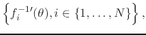
First of all, let us describe, in general lines, the algorithm we propose
to use in order to determine an inner analytic function that corresponds
to a given non-integrable real function. Given a non-integrable real
function ![]() , which is however locally integrable almost
everywhere, and whose hard singularities have a finite maximum degree of
hardness
, which is however locally integrable almost
everywhere, and whose hard singularities have a finite maximum degree of
hardness ![]() , we sectionally integrate it
, we sectionally integrate it ![]() times. Since by hypothesis
all the non-integrable singularities of
times. Since by hypothesis
all the non-integrable singularities of ![]() have degrees of
hardness of at most
have degrees of
hardness of at most ![]() , the resulting function
, the resulting function
![]() is
in fact an integrable one on the whole unit circle. Therefore, we may use
it to construct the corresponding inner analytic function, which we will
name
is
in fact an integrable one on the whole unit circle. Therefore, we may use
it to construct the corresponding inner analytic function, which we will
name
![]() , using the construction presented in [#!CAoRFI!#].
Having this inner analytic function, we then calculate its
, using the construction presented in [#!CAoRFI!#].
Having this inner analytic function, we then calculate its ![]() angular derivative, in order to obtain
angular derivative, in order to obtain ![]() , which is the inner analytic
function that corresponds to the non-integrable real function
, which is the inner analytic
function that corresponds to the non-integrable real function ![]() .
However, the
.
However, the ![]() -fold angular differentiation process produces only the
proper inner analytic function
-fold angular differentiation process produces only the
proper inner analytic function ![]() associated to
associated to ![]() , and
therefore produces
, and
therefore produces ![]() only up to an overall constant related to
the whole unit circle, as we will soon see. Of course this scheme will
succeed if and only if the non-integrable singular points of
only up to an overall constant related to
the whole unit circle, as we will soon see. Of course this scheme will
succeed if and only if the non-integrable singular points of ![]() all have finite degrees of hardness, with a maximum value of
all have finite degrees of hardness, with a maximum value of ![]() .
.
In this section we will prove the following theorem.
Before we attempt to prove the theorem, let us establish some notation for
a sectionally defined real function ![]() , that will be similar to
the one adopted for the piecewise polynomial functions discussed
in [#!CAoRFII!#], which is also given in Equation (6).
Since a non-integrable real function
, that will be similar to
the one adopted for the piecewise polynomial functions discussed
in [#!CAoRFII!#], which is also given in Equation (6).
Since a non-integrable real function ![]() which is locally
integrable almost everywhere is not defined at the singular points
corresponding to the angles
which is locally
integrable almost everywhere is not defined at the singular points
corresponding to the angles ![]() , for
, for
![]() , it is
in fact only sectionally defined, in
, it is
in fact only sectionally defined, in ![]() open intervals between
consecutive singularities, as given in Equation (5). Let us
therefore specify the definition of
open intervals between
consecutive singularities, as given in Equation (5). Let us
therefore specify the definition of ![]() as a set of
as a set of ![]() functions
functions ![]() defined on the
defined on the ![]() sections
sections
![]() ,
,
| (11) |
where, as before, we adopt the convention that every section
![]() is numbered after the singular point
is numbered after the singular point
![]() at its left end.
at its left end.
As a preliminary to the proof of the theorem, some considerations are in
order, regarding the multiple sectional integration of such non-integrable
functions. Note that, if ![]() is locally integrable almost
everywhere, then it is integrable within each one of the
is locally integrable almost
everywhere, then it is integrable within each one of the ![]() open
intervals that define the sections. More precisely, it is integrable on
every closed interval contained within one of these open intervals. In
terms of the sectional functions, since
open
intervals that define the sections. More precisely, it is integrable on
every closed interval contained within one of these open intervals. In
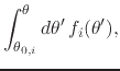
terms of the sectional functions, since ![]() is integrable
within its section, we may define a piecewise primitive for
is integrable
within its section, we may define a piecewise primitive for ![]() ,
by simply integrating each function
,
by simply integrating each function ![]() within the
corresponding open interval, starting at some arbitrary reference point
within the
corresponding open interval, starting at some arbitrary reference point
![]() strictly within that open interval. This will define the
piecewise primitive
strictly within that open interval. This will define the
piecewise primitive
 |
|||
 |
(12) |
where we have that
![]() and that
and that
![]() . Note that, since
. Note that, since ![]() is integrable on every closed interval contained within its section, it
follows that
is integrable on every closed interval contained within its section, it
follows that
![]() is limited on these closed
intervals, and therefore is also integrable on them. Therefore, this
process of sectional integration of the sectional functions can be
iterated indefinitely. If we iterate this process of sectional
integration, we obtain further piecewise primitives
is limited on these closed
intervals, and therefore is also integrable on them. Therefore, this
process of sectional integration of the sectional functions can be
iterated indefinitely. If we iterate this process of sectional
integration, we obtain further piecewise primitives
![]() ,
,
![]() , and so on. Note also that,
during this process of multiple sectional integration, some non-integrable
singularities, having a lower degree of hardness, may become integrable
before the others. In this case we might ignore the singularities which
became integrable, from that point on in the multiple integration process,
which therefore effectively reduces the number of sections, but for
simplicity we choose not to do that, and thus to keep the set of sections
constant. Note that, in any case, we do continue the process of sectional
integration until all the singularities have become integrable, of
course.
, and so on. Note also that,
during this process of multiple sectional integration, some non-integrable
singularities, having a lower degree of hardness, may become integrable
before the others. In this case we might ignore the singularities which
became integrable, from that point on in the multiple integration process,
which therefore effectively reduces the number of sections, but for
simplicity we choose not to do that, and thus to keep the set of sections
constant. Note that, in any case, we do continue the process of sectional
integration until all the singularities have become integrable, of
course.
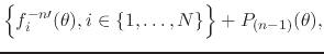
Although for definiteness we are integrating from some particular
reference points ![]() within each section, our objective here is
actually to construct primitives, and therefore we may ignore the
particular values chosen for
within each section, our objective here is
actually to construct primitives, and therefore we may ignore the
particular values chosen for ![]() if at each step in this
iterative process we add an arbitrary integration constant to the
primitive in each section, so that after
if at each step in this
iterative process we add an arbitrary integration constant to the
primitive in each section, so that after ![]() such successive integrations
a polynomial of degree
such successive integrations
a polynomial of degree ![]() , with
, with ![]() arbitrary coefficients, will have
been added to the
arbitrary coefficients, will have
been added to the ![]() primitive in the
primitive in the ![]() section. We
will express this as follows,
section. We
will express this as follows,
 |
|||
 |
|||
 |
(13) |
where
![]() is the most general piecewise
is the most general piecewise ![]() primitive of
primitive of ![]() ,
,
![]() is an arbitrary
is an arbitrary
![]() primitive of
primitive of ![]() in the
in the ![]() section,
section,
![]() is an arbitrary polynomial of order
is an arbitrary polynomial of order ![]() in the
in the
![]() section, and
section, and
![]() is a piecewise polynomial
function of order
is a piecewise polynomial
function of order ![]() , containing therefore
, containing therefore ![]() arbitrary constants in
each section. Note that
arbitrary constants in
each section. Note that
![]() is always an integrable real
function. Note also that, upon subsequent
is always an integrable real
function. Note also that, upon subsequent ![]() -fold differentiation of
-fold differentiation of
![]() with respect to
with respect to ![]() , all the arbitrary
constants that were added during the multiple integration process are then
eliminated, the arbitrary polynomials vanish from the result, and we thus
get back the original function
, all the arbitrary
constants that were added during the multiple integration process are then
eliminated, the arbitrary polynomials vanish from the result, and we thus
get back the original function ![]() , within the open intervals that
constitute the sections,
, within the open intervals that
constitute the sections,
Finally, we must emphasize some facts about the behavior of the
correspondence between inner analytic functions an integrable real
functions under the respective operations of differentiation and
integration, that take us along the corresponding integral-differential
chain. First, let us recall that, as we saw in [#!CAoRFI!#], both angular
differentiation and angular integration produce only proper inner
analytic functions, and thus always result in null Taylor coefficients
![]() , and thus in null Fourier coefficients
, and thus in null Fourier coefficients ![]() . Therefore,
when we use angular integration and differentiation in our algorithm, we
lose all information about these two
. Therefore,
when we use angular integration and differentiation in our algorithm, we
lose all information about these two ![]() coefficients. Second, as we
also saw in [#!CAoRFI!#], the integration on
coefficients. Second, as we
also saw in [#!CAoRFI!#], the integration on ![]() implies that the
resulting Fourier coefficient
implies that the
resulting Fourier coefficient ![]() becomes indeterminate due to
the presence of an arbitrary integration constant. It is due to this that
we must add arbitrary constants during the process of multiple sectional
integration, thus generating the arbitrary piecewise polynomial real
function
becomes indeterminate due to
the presence of an arbitrary integration constant. It is due to this that
we must add arbitrary constants during the process of multiple sectional
integration, thus generating the arbitrary piecewise polynomial real
function
![]() .
.
At this point, let us review the algorithm we are to use here. First,
starting from the non-integrable real function ![]() we go
we go ![]() steps
along the integration direction of the integral-differential chain, using
sectional integration on
steps
along the integration direction of the integral-differential chain, using
sectional integration on ![]() on the unit circle. This produces the
on the unit circle. This produces the
![]() -fold piecewise primitive
-fold piecewise primitive
![]() containing the
arbitrary piecewise polynomial real function
containing the
arbitrary piecewise polynomial real function
![]() . From the
globally integrable real function
. From the
globally integrable real function
![]() we then construct
the inner analytic function
we then construct
the inner analytic function
![]() , using the construction
presented in [#!CAoRFI!#]. We then come back in the differentiation
direction of the integral-differential chain the same number of steps,
using this time angular differentiation of the inner analytic functions
within the open unit disk. This produces an inner analytic function
associated to
, using the construction
presented in [#!CAoRFI!#]. We then come back in the differentiation
direction of the integral-differential chain the same number of steps,
using this time angular differentiation of the inner analytic functions
within the open unit disk. This produces an inner analytic function
associated to ![]() , except for its coefficient
, except for its coefficient ![]() , which means
that we recover only a proper inner analytic function, given that it is
the result of a series of angular differentiations, and we will therefore
denote this function by
, which means
that we recover only a proper inner analytic function, given that it is
the result of a series of angular differentiations, and we will therefore
denote this function by
![]() . Since this is equivalent to differentiation with
respect to
. Since this is equivalent to differentiation with
respect to ![]() of the piecewise polynomial real function
of the piecewise polynomial real function
![]() , it completely eliminates this function within the
open intervals that constitute the sections. However, it also produces the
superposition of a set of delta ``functions'' and derivatives of delta
``functions'' with support on the singular points between successive
sections.
, it completely eliminates this function within the
open intervals that constitute the sections. However, it also produces the
superposition of a set of delta ``functions'' and derivatives of delta
``functions'' with support on the singular points between successive
sections.
Thus we must conclude that this algorithm necessarily results in an
indeterminate Taylor coefficient ![]() of the inner analytic function
of the inner analytic function
![]() which corresponds to the real function
which corresponds to the real function ![]() , so that we
recover only the corresponding proper inner analytic function
, so that we
recover only the corresponding proper inner analytic function ![]() ,
and therefore it results in an equally indeterminate Fourier coefficients
,
and therefore it results in an equally indeterminate Fourier coefficients
![]() related to the real function
related to the real function ![]() . Se see, therefore,
that in this paper we are compelled to relax, to some extent, and only
during the process of construction of the inner analytic functions, the
correspondence between the real functions and these inner analytic
functions, considering only proper inner analytic functions, and accepting
the fact that they will correspond to the non-integrable real functions
only up to a global constant over the whole unit circle. Once the proper
inner analytic function
. Se see, therefore,
that in this paper we are compelled to relax, to some extent, and only
during the process of construction of the inner analytic functions, the
correspondence between the real functions and these inner analytic
functions, considering only proper inner analytic functions, and accepting
the fact that they will correspond to the non-integrable real functions
only up to a global constant over the whole unit circle. Once the proper
inner analytic function ![]() corresponding to a non-integrable real
function
corresponding to a non-integrable real
function ![]() has been determined, the relation will be written as
has been determined, the relation will be written as
| (14) |
where ![]() is a real constant, which can be determined afterwards,
by the simple comparison of the known value of the real part
is a real constant, which can be determined afterwards,
by the simple comparison of the known value of the real part
![]() of
of ![]() and the known value of
and the known value of ![]() , at any
point
, at any
point ![]() on the unit circle where they do not have hard
singularities. If
on the unit circle where they do not have hard
singularities. If ![]() is such a point, then we have that
is such a point, then we have that
![]() . Once the coefficient
. Once the coefficient
![]() is thus determined, this finally determines completely the
inner analytic function
is thus determined, this finally determines completely the
inner analytic function ![]() that corresponds to
that corresponds to ![]() ,
,
| (15) |
We are now ready to prove the theorem.
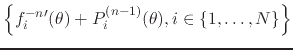
In order to prove the theorem, our first task is to show that we can
obtain an inner analytic function ![]() from the non-integrable real
function
from the non-integrable real
function ![]() , which is assumed to be locally integrable almost
everywhere. Consider that we execute the iterative piecewise integration
process described before
, which is assumed to be locally integrable almost
everywhere. Consider that we execute the iterative piecewise integration
process described before ![]() times on
times on ![]() , where
, where ![]() is the
maximum among all the degrees of hardness of the non-integrable hard
singularities involved. By doing this we generate a real function
is the
maximum among all the degrees of hardness of the non-integrable hard
singularities involved. By doing this we generate a real function
![]() which has only soft or at most borderline hard
singularities on the unit circle, and which is therefore integrable on the
whole unit circle.
which has only soft or at most borderline hard
singularities on the unit circle, and which is therefore integrable on the
whole unit circle.
It follows therefore that we may determine its set of Fourier
coefficients, as was done in [#!CAoRFI!#], which we will name
![]() ,
,
![]() and
and
![]() , for
, for
![]() . From this set of Fourier coefficients we
may then define, again as was done in [#!CAoRFI!#], the complex Taylor
coefficients
. From this set of Fourier coefficients we
may then define, again as was done in [#!CAoRFI!#], the complex Taylor
coefficients ![]() , for
, for
![]() . From
these coefficients we may then determine the unique inner analytic
function that corresponds to the
. From
these coefficients we may then determine the unique inner analytic
function that corresponds to the ![]() piecewise primitive
piecewise primitive
![]() , which we will name
, which we will name
![]() .
Note that we may use this notation unequivocally because every proper
inner analytic function belongs to an infinite integral-differential
chain, extending indefinitely to either side, so that we know that there
exists in fact a proper inner analytic function
.
Note that we may use this notation unequivocally because every proper
inner analytic function belongs to an infinite integral-differential
chain, extending indefinitely to either side, so that we know that there
exists in fact a proper inner analytic function ![]() associated to
associated to
| (16) |
namely its ![]() angular derivative. As we have shown
in [#!CAoRFI!#], from the
angular derivative. As we have shown
in [#!CAoRFI!#], from the
![]() limit to the unit circle of
the real part
limit to the unit circle of
the real part
![]() of the inner analytic function
of the inner analytic function
![]() we can recover the integrable real function
we can recover the integrable real function
![]() , almost everywhere in its domain of definition. We
thus have the correspondence for the integrable real function
, almost everywhere in its domain of definition. We
thus have the correspondence for the integrable real function
| (17) |
Having done this, we now take the ![]() angular derivative of the
inner analytic function
angular derivative of the
inner analytic function
![]() , thus obtaining a proper inner
analytic function
, thus obtaining a proper inner
analytic function
![]() . Since
. Since ![]() angular differentiations of
angular differentiations of
![]() correspond to
correspond to ![]() differentiations with respect to
differentiations with respect to
![]() of
of
![]() , and thus completely eliminates the
piecewise polynomial real function
, and thus completely eliminates the
piecewise polynomial real function
![]() within the domain
of definition of
within the domain
of definition of ![]() , it follows that the function
, it follows that the function ![]() is a
proper inner analytic function corresponding to the non-integrable real
function
is a
proper inner analytic function corresponding to the non-integrable real
function ![]() . As discussed before, this correspondence is valid
only up to a global real constant yet to be determined, so that we may now
write
. As discussed before, this correspondence is valid
only up to a global real constant yet to be determined, so that we may now
write
| (18) |
where ![]() can then be determined as discussed before, by the
comparison between the real part
can then be determined as discussed before, by the
comparison between the real part
![]() of
of ![]() and
and
![]() at some particular point on the unit circle where they do not
have hard singularities. Having determined
at some particular point on the unit circle where they do not
have hard singularities. Having determined ![]() , and therefore
, and therefore
![]() , we may now define the inner analytic function that
corresponds to
, we may now define the inner analytic function that
corresponds to ![]() ,
,
| (19) |
so that we have the relation leading from ![]() to
to ![]()
| (20) |
This completes the first part of the proof of Theorem 1.
We must now prove that we can recover ![]() from the real part
from the real part
![]() of
of ![]() in the
in the
![]() limit. In order to do
this, we start from the fact that from [#!CAoRFI!#] we know this to be
true for the
limit. In order to do
this, we start from the fact that from [#!CAoRFI!#] we know this to be
true for the ![]() -fold primitives
-fold primitives
| (21) |
While the inner analytic function
![]() is given by the power
series
is given by the power
series
 |
(22) |
as we have shown in [#!CAoRFIII!#] the real function
![]() can be expressed almost everywhere as an regulated
Fourier series, even if the Fourier series itself diverges almost
everywhere,
can be expressed almost everywhere as an regulated
Fourier series, even if the Fourier series itself diverges almost
everywhere,
![\begin{displaymath}
f^{-n\prime}(\theta)
=
\frac{\alpha_{0}^{(-n)}}{2}
+
\l...
...(-n)}\cos(k\theta)
+
\beta_{k}^{(-n)}\sin(k\theta)
\right],
\end{displaymath}](img132.png) |
(23) |
where we have that
![]() and that
and that
![]() for
for
![]() . As we established in [#!CAoRFIII!#], since
the sequences of Fourier coefficients
. As we established in [#!CAoRFIII!#], since
the sequences of Fourier coefficients
![]() and
and
![]() are exponentially bounded, this series is absolutely
and uniformly convergent for
are exponentially bounded, this series is absolutely
and uniformly convergent for ![]() . As we saw in [#!CAoRFI!#], the
fact that we can recover
. As we saw in [#!CAoRFI!#], the
fact that we can recover
![]() as the
as the
![]() limit of the real part
limit of the real part
![]() of
of
![]() is
a consequence of the fact that the two real functions
is
a consequence of the fact that the two real functions
![]() and
and
![]() have exactly the same
set of Fourier coefficients. This, is turn, can be expressed as the
relations between the Taylor coefficients
have exactly the same
set of Fourier coefficients. This, is turn, can be expressed as the
relations between the Taylor coefficients ![]() associated to
associated to
![]() and the Fourier coefficients
and the Fourier coefficients
![]() and
and
![]() associated to
associated to ![]() , which have just been given
above.
, which have just been given
above.
Let us now prove that the correspondence between
![]() and
and
![]() implies the same
correspondence between
implies the same
correspondence between
![]() and
and
![]() , when we differentiate the two functions. We
can do this by just showing that the relations between the Taylor
coefficients and the Fourier coefficients are preserved by this process of
differentiation. If we just differentiate the inner analytic function
using angular differentiation we get
, when we differentiate the two functions. We
can do this by just showing that the relations between the Taylor
coefficients and the Fourier coefficients are preserved by this process of
differentiation. If we just differentiate the inner analytic function
using angular differentiation we get
 |
|||
 |
(24) |
from which we have for the Taylor coefficients
![]() , for
, for
![]() . Note that, since this
is a convergent power series, we can always differentiate it
term-by-term. If we now differentiate the real function using simple
differentiation with respect to
. Note that, since this
is a convergent power series, we can always differentiate it
term-by-term. If we now differentiate the real function using simple
differentiation with respect to ![]() we get
we get
![$\displaystyle \lim_{\rho\to 1_{(-)}}
\sum_{k=1}^{\infty}
\rho^{k}
\left[
k\,\beta_{k}^{(-n)}\cos(k\theta)
-
k\,\alpha_{k}^{(-n)}\sin(k\theta)
\right],$](img143.png) |
|||
![$\displaystyle \lim_{\rho\to 1_{(-)}}
\sum_{k=1}^{\infty}
\rho^{k}
\left[
\alpha_{k}^{(-n+1)}\cos(k\theta)
+
\beta_{k}^{(-n+1)}\sin(k\theta)
\right],$](img144.png) |
(25) |
from which we have for the corresponding Fourier coefficients that
![]() and also that
and also that
![]() , for
, for
![]() . Note that we have, in either case, that
. Note that we have, in either case, that
![]() and that
and that
![]() , so that the relation
between
, so that the relation
between ![]() and
and
![]() is in fact preserved. Note
also that, since this trigonometric series is uniformly convergent, and in
fact is the real part of a convergent complex power series, we may
differentiate it term-by-term so long as the series thus obtained is also
convergent. Since the Fourier coefficients
is in fact preserved. Note
also that, since this trigonometric series is uniformly convergent, and in
fact is the real part of a convergent complex power series, we may
differentiate it term-by-term so long as the series thus obtained is also
convergent. Since the Fourier coefficients
![]() and
and
![]() , which increase at most as a power of
, which increase at most as a power of ![]() when
when
![]() , are thus seen to be exponentially bounded, this implies that
the series thus obtained is also absolutely and uniformly convergent, as
we have shown in [#!CAoRFIII!#]. Therefore, we are justified in
differentiating the original series term-by-term. We therefore have the
relation between the Taylor coefficients
, are thus seen to be exponentially bounded, this implies that
the series thus obtained is also absolutely and uniformly convergent, as
we have shown in [#!CAoRFIII!#]. Therefore, we are justified in
differentiating the original series term-by-term. We therefore have the
relation between the Taylor coefficients
![]() and the Fourier
coefficients
and the Fourier
coefficients
![]() and
and
![]() ,
,
![$\displaystyle \mbox{\boldmath$\imath$}k
\left[
\alpha_{k}^{(-n)}
-
\mbox{\boldmath$\imath$}
\beta_{k}^{(-n)}
\right]$](img157.png) |
|||
![$\displaystyle \mbox{\boldmath$\imath$}k
\left[
-\,
\frac{1}{k}\,
\beta_{k}^{(-n+1)}
-
\mbox{\boldmath$\imath$}\,
\frac{1}{k}\,
\alpha_{k}^{(-n+1)}
\right]$](img158.png) |
|||
| (26) |
We see therefore that we indeed have that the relation between
![]() ,
,
![]() and
and
![]() , for
, for
![]() , is also preserved,
, is also preserved,
| (27) |
which thus establishes the correspondence for the first derivatives. We
may now extend this argument to subsequent derivatives, from
![]() and
and
![]() all the way to
all the way to ![]() and
and ![]() , by finite induction. Therefore, let us assume the result
for the case
, by finite induction. Therefore, let us assume the result
for the case ![]() and show that this implies that it is also valid for
the case
and show that this implies that it is also valid for
the case ![]() . We assume therefore that we have
. We assume therefore that we have
| (28) |
for some positive value of ![]() , where the functions are expressed as the
corresponding series
, where the functions are expressed as the
corresponding series
 |
|||
![$\displaystyle \lim_{\rho\to 1_{(-)}}
\sum_{k=1}^{\infty}
\rho^{k}
\left[
\alpha_{k}^{(-n+i)}\cos(k\theta)
+
\beta_{k}^{(-n+i)}\sin(k\theta)
\right].$](img169.png) |
(29) |
We may now differentiate either series term-by-term, which we may do for the same reasons as before, thus obtaining
 |
|||
![$\displaystyle \lim_{\rho\to 1_{(-)}}
\sum_{k=1}^{\infty}
\rho^{k}
\left[
k\,\beta_{k}^{(-n+i)}\cos(k\theta)
-
k\,\alpha_{k}^{(-n+i)}\sin(k\theta)
\right],$](img173.png) |
(30) |
so that we have for the coefficients for the case ![]()
| (31) |
for
![]() . Using now the relations between the
coefficients for the case
. Using now the relations between the
coefficients for the case ![]() we have
we have
![$\displaystyle \mbox{\boldmath$\imath$}k
\left[
\alpha_{k}^{(-n+i)}
-
\mbox{\boldmath$\imath$}
\beta_{k}^{(-n+i)}
\right]$](img181.png) |
|||
![$\displaystyle \mbox{\boldmath$\imath$}k
\left[
-\,
\frac{1}{k}\,
\beta_{k}^{(-n+i+1)}
-
\mbox{\boldmath$\imath$}\,
\frac{1}{k}\,
\alpha_{k}^{(-n+i+1)}
\right]$](img182.png) |
|||
| (32) |
for
![]() , thus showing that the relation between
the coefficients is in fact preserved, where we recall that the
, thus showing that the relation between
the coefficients is in fact preserved, where we recall that the ![]() coefficients are always zero during this process. This is therefore true
for all possible multiple derivatives, all the way to infinity, and in
particular it is true for
coefficients are always zero during this process. This is therefore true
for all possible multiple derivatives, all the way to infinity, and in
particular it is true for ![]() , that is, for the coefficients of
, that is, for the coefficients of ![]() and
and ![]() . In order to complete the proof in this case all we have
to do is to consider the real function
. In order to complete the proof in this case all we have
to do is to consider the real function
| (33) |
where
| (34) |
Since the expression of the Fourier coefficients is linear on the
functions, and since ![]() and
and ![]() have exactly the same
set of Fourier coefficients, it is clear that all the Fourier coefficients
of
have exactly the same
set of Fourier coefficients, it is clear that all the Fourier coefficients
of ![]() are zero. Therefore, for the real function
are zero. Therefore, for the real function ![]() we
have that
we
have that ![]() for all
for all ![]() , and thus the inner analytic function that
corresponds to
, and thus the inner analytic function that
corresponds to ![]() is the identically null complex function
is the identically null complex function
![]() . This is an inner analytic function which is, in
fact, analytic over the whole complex plane, and which, in particular, is
zero over the unit circle, so that we have
. This is an inner analytic function which is, in
fact, analytic over the whole complex plane, and which, in particular, is
zero over the unit circle, so that we have
![]() , since the
identically zero real function is the only integrable real function
without removable singularities that corresponds to the identically zero
inner analytic function, due to the completeness of the Fourier basis, as
was shown in [#!CAoRFIII!#]. Note, in particular, that the
, since the
identically zero real function is the only integrable real function
without removable singularities that corresponds to the identically zero
inner analytic function, due to the completeness of the Fourier basis, as
was shown in [#!CAoRFIII!#]. Note, in particular, that the
![]() limits exist at all points of the unit circle in the case
of the inner analytic function associated to
limits exist at all points of the unit circle in the case
of the inner analytic function associated to ![]() . Since both
. Since both
![]() and
and ![]() have non-integrable hard singularities at
isolated points on the unit circle, we can conclude only that
have non-integrable hard singularities at
isolated points on the unit circle, we can conclude only that
| (35) |
almost everywhere on the unit circle, or everywhere in the domain of
definition of ![]() , which therefore excludes all the points where
the function has hard singularities. Note that the domain of definition of
, which therefore excludes all the points where
the function has hard singularities. Note that the domain of definition of
![]() is the same as that of
is the same as that of ![]() , because any hard
singularities that may have been softened in the process of iterative
integration, during the construction of
, because any hard
singularities that may have been softened in the process of iterative
integration, during the construction of ![]() , will have been hardened
again in the corresponding process of iterative differentiation. We have
therefore the complete correspondence
, will have been hardened
again in the corresponding process of iterative differentiation. We have
therefore the complete correspondence
| (36) |
The inner analytic function ![]() represents the non-integrable real
function
represents the non-integrable real
function ![]() exactly in the same way as that which was established
for integrable real functions in [#!CAoRFI!#]. Note that this proof
establishes that the correspondence between the inner analytic functions
and the real functions is also valid for all the intermediate cases, from
exactly in the same way as that which was established
for integrable real functions in [#!CAoRFI!#]. Note that this proof
establishes that the correspondence between the inner analytic functions
and the real functions is also valid for all the intermediate cases, from
![]() and
and
![]() to
to ![]() and
and ![]() .
This completes the second part of the proof of Theorem 1.
.
This completes the second part of the proof of Theorem 1.
Let us once more draw attention to the fact that the inner analytic
function ![]() produced in the way described above, while it does
correspond to the non-integrable real function
produced in the way described above, while it does
correspond to the non-integrable real function ![]() , is not
unique. One can add to it any linear combination of inner analytic
functions that correspond to singular distributions with their
singularities at the singular points on the unit circle corresponding to
the angles
, is not
unique. One can add to it any linear combination of inner analytic
functions that correspond to singular distributions with their
singularities at the singular points on the unit circle corresponding to
the angles
![]() , without changing the fact
that the non-integrable real function
, without changing the fact
that the non-integrable real function ![]() is still recovered as
the
is still recovered as
the
![]() limit of the real part of the new inner analytic
function obtained in this way, at all points where it is well defined.
limit of the real part of the new inner analytic
function obtained in this way, at all points where it is well defined.
Given the inner analytic function ![]() that was obtained from
that was obtained from
![]() by the process described above, one can then consider defining
from it a reduced inner analytic function
by the process described above, one can then consider defining
from it a reduced inner analytic function ![]() that represents
the non-integrable real function in a unique way, without the
superposition of any singular distributions. If the
that represents
the non-integrable real function in a unique way, without the
superposition of any singular distributions. If the ![]() singular points of
singular points of
![]() are examined in order to determine the existence there of singular
distributions, and since each one of these singular distributions is
represented by a known unique inner analytic function of its own, as was
shown in [#!CAoRFII!#], one can simply subtract from
are examined in order to determine the existence there of singular
distributions, and since each one of these singular distributions is
represented by a known unique inner analytic function of its own, as was
shown in [#!CAoRFII!#], one can simply subtract from ![]() the
appropriate linear combination of inner analytic functions of the singular
distributions present, in order to obtain an inner analytic function that
represents the non-integrable real function
the
appropriate linear combination of inner analytic functions of the singular
distributions present, in order to obtain an inner analytic function that
represents the non-integrable real function ![]() alone, without any
singular distributions superposed to it.
alone, without any
singular distributions superposed to it.
The simplest way to do this is to examine the result of every angular
differentiation during the process leading from
![]() to
to
![]() . At each step one can verify whether or not the angular
differentiation has generated one or more Dirac delta ``functions'' at
some of the singular points. This is a simple thing to verify, because the
occurrence of a delta ``function'' at a certain point is always preceded
by the occurrence of a finite discontinuity of the real function at that
point. This can also be done by the determination of the type and
orientation of the singularities at these points, since the Dirac delta
``functions'' are associated to inner analytic functions with simple poles
that have a specific orientation with respect to the unit circle. One can
then subtract from the proper inner analytic function obtained at that
point in the iterative differentiation process the inner analytic
functions corresponding to the delta ``functions'' at the appropriate
points. By doing this one guarantees that no derivatives of delta
``functions'' will ever arise during the process of multiple
differentiation. After one determines
. At each step one can verify whether or not the angular
differentiation has generated one or more Dirac delta ``functions'' at
some of the singular points. This is a simple thing to verify, because the
occurrence of a delta ``function'' at a certain point is always preceded
by the occurrence of a finite discontinuity of the real function at that
point. This can also be done by the determination of the type and
orientation of the singularities at these points, since the Dirac delta
``functions'' are associated to inner analytic functions with simple poles
that have a specific orientation with respect to the unit circle. One can
then subtract from the proper inner analytic function obtained at that
point in the iterative differentiation process the inner analytic
functions corresponding to the delta ``functions'' at the appropriate
points. By doing this one guarantees that no derivatives of delta
``functions'' will ever arise during the process of multiple
differentiation. After one determines ![]() at the last step of the
process, this will lead to a reduced inner analytic function
at the last step of the
process, this will lead to a reduced inner analytic function ![]() which includes no singular distributions at all, and that hence
corresponds to
which includes no singular distributions at all, and that hence
corresponds to ![]() in a unique and simple way,
in a unique and simple way,
| (37) |
that does not include the superposition of any singular distributions with support on the singular points between successive sections.