Representation of Integrable Real Functions

In this section we will establish the relation between integrable real functions and inner analytic functions. When we discuss real functions in this paper, some properties will be globally assumed for these functions. These are rather weak conditions to be imposed on these functions, that will be in force throughout this paper. It is to be understood, without any need for further comment, that these conditions are valid whenever real functions appear in the arguments. These weak conditions certainly hold for any integrable real functions that are obtained as restrictions of corresponding inner analytic functions to the unit circle. The most basic condition is that the real functions must be measurable in the sense of Lebesgue, with the usual Lebesgue measure [#!RARudin!#,#!RARoyden!#]. In essence, this is basic infrastructure to allow the functions to be integrable.

In order to discuss the other global conditions, we must first discuss the classification of singularities of a real function. The concept of a singularity itself is the same as that for a complex function, namely a point where the function is not analytic. The concept of a removable singularity is well-known for analytic functions in the complex plane. What we mean by a removable singularity in the case of real functions on the unit circle is a singular point such that both lateral limits of the function to that point exist and result in the same real value, but where the function has been arbitrarily defined to have some other real value. This is therefore a point were the function can be redefined by continuity, resulting in a continuous function at that point. The concepts of soft and hard singularities are carried in a straightforward way from the case of complex functions, discussed in Section 2, to that of real functions. The only difference is that the concept of the limit of the function to the point is now taken to be the real one, along the unit circle.

The second global condition we will impose is that the functions have no removable singularities. Since they can be easily eliminated, these are trivial singularities, which we will simply rule out of our discussions in this paper. Although the presence of even a denumerably infinite set of such trivial singularities does not significantly affect the results to be presented here, their elimination does significantly simplify the arguments to be presented. It is for this reason, that is, for the sake of simplicity, that we rule out such irrelevant singularities. In addition to this we will require, as our third an last global condition, that the number of hard singularities be finite, and hence that they be all isolated from one another. There will be no limitation on the number of soft singularities. In terms of the more immediate characteristics of the real functions, the relevant requirement is that the number of singular points where a given real function diverges to infinity be finite.

In this section we will prove the following theorem.

Theorem 1   : Every integrable real function defined on a finite interval can be represented by an inner analytic function, and can be recovered almost everywhere by means of the limit to the unit circle of the real part of that inner analytic function.

Given an arbitrary real function defined within an arbitrary finite closed interval, it can always be mapped to a real function within the periodic interval $[-\pi,\pi]$, by a simple linear change of variables, so it suffices for our purposes here to examine only the set of real functions $f(\theta)$ defined in this standard interval. The interval is then mapped onto the unit circle of the complex $z$ plane. What happens to the values of the function at the two ends of the interval when one does this is irrelevant for our purposes here, but for definiteness we may think that one attributes to the function at the point $z=-1$ the arithmetic average of the values of the function at the two ends of the periodic interval. The further requirements to be imposed on these functions are still quite weak, namely no more than that they be Lebesgue-integrable in the periodic interval, so that one can attribute to them a set of Fourier coefficients [#!FSchurchill!#].

Since for Lebesgue-measurable functions defined within a compact interval plain integrability and absolute integrability are equivalent requirements [#!RARudin!#,#!RARoyden!#], we may assume that the functions are absolutely integrable, without loss of generality. Note that the functions do not have to be differentiable or even continuous. They may also be unlimited, possibly diverging to infinity at some singular points, so long as they are absolutely integrable. This means, of course, that any hard singularities that they may have at isolated points must be integrable singularities, which we may thus characterize as borderline hard singularities, in a real sense of the term. This means, in turn, that although the functions may diverge to infinity at isolated points, their pairs of asymptotic integrals around these points must still exist and be finite real numbers.

This in turn means that these borderline hard singularities must be surrounded by open intervals where there are no other borderline hard singularities, so that the asymptotic integrals around the singular points can be well defined and finite. It follows that any existing borderline hard singularities must be isolated from any other borderline hard singularities. Note that they do not really have to be isolated singularities in the usual, strict sense of complex analysis, which would require that they be isolated from all other singularities. All that is required is that the borderline hard singularities be isolated from each other. Hence the requirement that the number of hard singularities be finite. Note also that one can have any number of soft singularities, even an infinite number of them. As we pointed out before, in terms of the properties of the real functions $f(\theta)$, the important requirement is that the number of singular points on the unit circle where a given real function diverges to infinity be finite.

Proof 1.1   :

With all these preliminaries stated, the first thing that we must do here is, given an arbitrary integrable real function $f(\theta)$ defined within the periodic interval $[-\pi,\pi]$, to build from it an analytic function $w(z)$ within the open unit disk of the complex plane. For this purpose we will use the Fourier coefficients of the given real function. The Fourier coefficients [#!FSchurchill!#] are defined by

$$\alpha_{0} = \frac{1}{\pi} \int_{-\pi}^{\pi}d\theta\, f(\theta),$$

$$\alpha_{k} = \frac{1}{\pi} \int_{-\pi}^{\pi}d\theta\, \cos(k\theta)f(\theta),$$

$$\beta_{k} = \frac{1}{\pi} \int_{-\pi}^{\pi}d\theta\, \sin(k\theta)f(\theta),$$ (20)

where the set of functions $\left\{\rule{0em}{2ex}1,\cos(k\theta),\sin(k\theta), k\in\{1,2,3,\ldots,\infty\}\right\}$, constitutes the Fourier basis of functions. Since $f(\theta)$ is absolutely integrable, we have that

$$\int_{-\pi}^{\pi}d\theta\, \vert f(\theta)\vert = 2\pi M,$$ (21)

where $M$ is a positive and finite real number, namely the average value, on the periodic interval $[-\pi,\pi]$, of the absolute value of the function. If we use the triangle inequalities, it follows therefore that $\alpha_{0}$ exists and that it satisfies

$$\vert\alpha_{0}\vert \leq \frac{1}{\pi} \int_{-\pi}^{\pi}d\theta\, \vert f(\theta)\vert$$

$$= 2M,$$ (22)

that is, it is limited by $2M$. Since the elements of the Fourier basis are all limited smooth functions, and using again the triangle inequalities, it now follows that all other Fourier coefficients also exist, and are also all limited by $2M$,

$$\vert\alpha_{k}\vert \leq \frac{1}{\pi} \int_{-\pi}^{\pi}d\theta\, \vert\cos(k\theta)\vert\vert f(\theta)\vert$$

$$\leq \frac{1}{\pi} \int_{-\pi}^{\pi}d\theta\, \vert f(\theta)\vert$$

$$= 2M,$$

$$\vert\beta_{k}\vert \leq \frac{1}{\pi} \int_{-\pi}^{\pi}d\theta\, \vert\sin(k\theta)\vert\vert f(\theta)\vert$$

$$\leq \frac{1}{\pi} \int_{-\pi}^{\pi}d\theta\, \vert f(\theta)\vert$$

$$= 2M,$$ (23)

for all $k$, since the absolute values of the sines and cosines are limited by one. Given that we have the coefficients $\alpha_{k}$ and $\beta_{k}$, the construction of the corresponding inner analytic function is now straightforward. We simply define the set of complex coefficients

$$c_{0} = \frac{1}{2}\,\alpha_{0},$$

$$c_{k} = \alpha_{k} - \mbox{\boldmath$\imath$}\beta_{k},$$ (24)

for $k\in\{1,2,3,\ldots,\infty\}$. Note that these coefficients are all limited by $4M$, since, using once more the triangle inequalities, we have

$$\vert c_{0}\vert = \frac{1}{2}\,\vert\alpha_{0}\vert$$

$$\leq M,$$

$$\vert c_{k}\vert \leq \vert\alpha_{k}\vert + \vert\beta_{k}\vert$$

$$\leq 4M.$$ (25)

We now define a complex variable $z$ associated to $\theta$, using an auxiliary positive real variable $\rho\geq 0$,

$$z = \rho\,{\rm e}^{\mbox{\boldmath\scriptsize$\imath$}\theta},$$ (26)

where $(\rho,\theta)$ are polar coordinates in the complex $z$ plane. We then construct the following power series around the origin $z=0$,

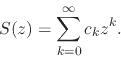$$S(z) = \sum_{k=0}^{\infty} c_{k}z^{k}.$$ (27)

According to the theorems of complex analysis [#!CVchurchill!#], where this power series converges in the complex $z$ plane, it converges absolutely and uniformly to an analytic function $w(z)$. It then follows that $S(z)$ is in fact the Taylor series of $w(z)$ around $z=0$. We must now establish that this series converges within the open unit disk, whatever the values of the Fourier coefficients, given only that they are all limited by $4M$. In order to do this we will first prove that the series $S(z)$ is absolutely convergent, that is, we will establish the convergence of the corresponding series of absolute values

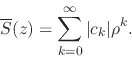$$\overline{S}(z) = \sum_{k=0}^{\infty} \vert c_{k}\vert\rho^{k}.$$ (28)

Let us now consider the partial sums of this real series, and replace the absolute values of the coefficients by their common upper bound,

$$\overline{S}_{n}(z) = \sum_{k=0}^{n} \vert c_{k}\vert\rho^{k}$$

$$\leq 4M \sum_{k=0}^{n} \rho^{k},$$ (29)

where $n\in\{0,1,2,3,\ldots,\infty\}$. This is now the sum of a geometric progression, so that we have

$$\overline{S}_{n}(z) \leq 4M\, \frac{1-\rho^{n+1}}{1-\rho}.$$ (30)

For $\rho<1$ we may now take the $n\to\infty$ limit of the right-hand side, without violating the inequality, so that we get the sum of a geometric series,

$$\overline{S}_{n}(z) \leq \frac{4M}{1-\rho}.$$ (31)

For $\rho<1$ the right-hand side is now a positive upper bound for all the partial sums of the series of absolute values. Therefore, since the sequence $\overline{S}_{n}(z)$ of partial sums is a monotonically increasing sequence of real numbers which is bounded from above, it now follows that this real sequence is necessarily a convergent one.

Therefore the series of absolute values $\overline{S}(z)$ is convergent on the open unit disk $\rho<1$, which in turn implies that the original series $S(z)$ is absolutely convergent on that same disk. This then implies that the series $S(z)$ is simply convergent on that same disk. Since $S(z)$ is a convergent power series, it converges to an analytic function on the open unit disk, which we may now name $w(z)$. Since this is an analytic function within the open unit disk, it is an inner analytic function, the one that corresponds to the real function $f(\theta)$ on the unit circle,

$$f(\theta) \longrightarrow w(z).$$ (32)

The coefficients $c_{k}$ are now recognized as the Taylor coefficients of the inner analytic function $w(z)$ with respect to the origin. We have therefore established that from any integrable real function $f(\theta)$ one can define a unique corresponding inner analytic function $w(z)$. This completes the first part of the proof of Theorem 1.

Next we must establish that $f(\theta)$ can be recovered as the limit $\rho\to 1_{(-)}$, from the open unit disk to the unit circle, of the real part of $w(z)$, so that we can establish the complete correspondence between the integrable real function and the inner analytic function,

$$f(\theta) \longleftrightarrow w(z).$$ (33)

Proof 1.2   :

We start by writing the coefficients $c_{k}$ in terms of $w(z)$ and discussing their dependence on $\rho$. Since the complex coefficients $c_{k}$ are the coefficients of the Taylor series of $w(z)$ around $z=0$, the Cauchy integral formulas of complex analysis, for the function $w(z)$ and its derivatives, written at $z=0$ for the $k^{\rm th}$ derivative of $w(z)$, tell us that we have

$$c_{k} = \frac{1}{2\pi\mbox{\boldmath$\imath$}} \oint_{C}dz\, \frac{w(z)}{z^{k+1}},$$ (34)

for all $k$, where $C$ is any simple closed curve within the open unit disk that contains the origin, which we may now take as a circle centered at $z=0$ with radius $\rho\in(0,1)$. We now note that, since $w(z)$ is analytic in the open unit disk, so that the explicit singularity at $z=0$ is the only singularity of the integrand on that disk, by the Cauchy-Goursat theorem the integral is independent of $\rho$ within the open unit disk, and therefore so are the complex coefficients $c_{k}$.

It thus follows that the coefficients $c_{k}$ are continuous functions of $\rho$ inside the open unit disk, and therefore that their $\rho\to 1_{(-)}$ limits exist and have those same constant values. Since we have the relations in Equation (24), the same is true for the Fourier coefficients $\alpha_{k}$ and $\beta_{k}$. On the other hand, by construction these are the same coefficients that were obtained from the real function $f(\theta)$ on the unit circle, and we may thus conclude that the coefficients $c_{k}$, $\alpha_{k}$ and $\beta_{k}$, for all $k$, are all constant with $\rho$ and therefore continuous functions of $\rho$ in the whole closed unit disk. This means that, at least in the case of the coefficients, the $\rho\to 1_{(-)}$ limit can be taken trivially.

Let us now establish the fact that $f(\theta)$ and the real part $u(1,\theta)$ of $w(z)$ at $\rho=1$ have exactly the same set of Fourier coefficients. We consider first the case of the coefficient $\alpha_{0}$. If we write the Cauchy integral formula in Equation (34) for the case $k=0$ we get

$$c_{0} = \frac{1}{2\pi\mbox{\boldmath$\imath$}} \oint_{C}dz\, \frac{w(z)}{z}.$$ (35)

Recalling that $c_{0}=\alpha_{0}/2$ and writing the integral on the circle of radius $\rho$ using the integration variable $\theta$ we get

$$\frac{\alpha_{0}}{2} = \frac{1}{2\pi} \int_{-\pi}^{\pi}d... ...\theta) + \mbox{\boldmath$\imath$} v(\rho,\theta) \right].$$ (36)

Since $\alpha_{0}$ is real, we conclude that the imaginary part in the right-hand side must be zero, and thus obtain

$$\alpha_{0} = \frac{1}{\pi} \int_{-\pi}^{\pi}d\theta\, u(\rho,\theta),$$ (37)

thus proving that $\alpha_{0}$, which is the $k=0$ Fourier coefficient of $f(\theta)$, is also the $k=0$ Fourier coefficient of $u(\rho,\theta)$, for any value of $\rho$, and thus is, in particular, the $k=0$ Fourier coefficient of $u(1,\theta)$. This is so because, since the $\rho\to 1_{(-)}$ limit of the coefficient $\alpha_{0}$ can be taken, so can the limit of the integral in the right-hand side. Note that this shows, in particular, that $u(1,\theta)$ is an integrable real function. In order to extend the analysis of the coefficients to the case $k>0$ we must first derive some preliminary relations. Consider therefore the following integral, on the same circuit $C$ we used in Equation (34),

$$\oint_{C}dz\, w(z)z^{k-1} = 0,$$ (38)

with $k>0$. The integral is zero by the Cauchy-Goursat theorem, since for $k\geq 1$ the integrand is analytic on the whole open unit disk. As before we write the integral on the circle of radius $\rho$ using the integration variable $\theta$, to get

$$\int_{-\pi}^{\pi}d\theta\, \left[ u(\rho,\theta)\cos(k\theta) - v(\rho,\theta)\sin(k\theta) \right] \hspace{1em}$$

$$+ \mbox{\boldmath$\imath$} \int_{-\pi}^{\pi}d\theta\, \left[ u(\rho,\theta)\sin(k\theta) + v(\rho,\theta)\cos(k\theta) \right] = 0.$$ (39)

We are therefore left with the two identities involving $u(\rho,\theta)$ and $v(\rho,\theta)$,

$$\int_{-\pi}^{\pi}d\theta\, u(\rho,\theta)\cos(k\theta) = \int_{-\pi}^{\pi}d\theta\, v(\rho,\theta)\sin(k\theta),$$

$$\int_{-\pi}^{\pi}d\theta\, u(\rho,\theta)\sin(k\theta) = - \int_{-\pi}^{\pi}d\theta\, v(\rho,\theta)\cos(k\theta),$$ (40)

which are valid for all $k>0$ and for all $\rho\in(0,1)$. If we now write the integrals of the Cauchy integral formulas in Equation (34) explicitly as integrals on $\theta$, we get

$$c_{k} = \frac{\rho^{-k}}{2\pi} \left\{ \int_{-\pi}^{\pi}d\theta\, \left[ u(\rho,\theta)\cos(k\theta) + v(\rho,\theta)\sin(k\theta) \right] \right.$$

$$\hspace{2.4em} \left. + \mbox{\boldmath$\imath$} \int_{-\pi}^{\pi... ...[ - u(\rho,\theta)\sin(k\theta) + v(\rho,\theta)\cos(k\theta) \right] \right\}.$$ (41)

Using the identities in Equation (40) in order to eliminate $v(\rho,\theta)$ in favor of $u(\rho,\theta)$ and recalling that $c_{k}=\alpha_{k}-\mbox{\boldmath$\imath$}\beta_{k}$ we get

$$\alpha_{k} - \mbox{\boldmath$\imath$} \beta_{k} = \fra... ...mbox{\boldmath$\imath$} u(\rho,\theta)\sin(k\theta) \right],$$ (42)

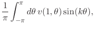
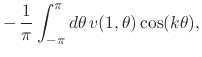
so that we have the relations for the Fourier coefficients,

$$\alpha_{k} = \frac{\rho^{-k}}{\pi} \int_{-\pi}^{\pi}d\theta\, u(\rho,\theta)\cos(k\theta),$$

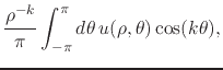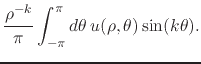$$\beta_{k} = \frac{\rho^{-k}}{\pi} \int_{-\pi}^{\pi}d\theta\, u(\rho,\theta)\sin(k\theta).$$ (43)

Since the $\rho\to 1_{(-)}$ limits of the coefficients in the left-hand sides can be taken, so can the $\rho\to 1_{(-)}$ limits of the integrals in the right-hand sides. Therefore, taking the limit we have for the Fourier coefficients,

$$\alpha_{k} = \frac{1}{\pi} \int_{-\pi}^{\pi}d\theta\, u(1,\theta)\cos(k\theta),$$

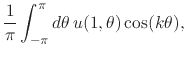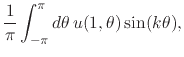$$\beta_{k} = \frac{1}{\pi} \int_{-\pi}^{\pi}d\theta\, u(1,\theta)\sin(k\theta),$$ (44)

thus completing the proof that the real functions $u(1,\theta)$ and $f(\theta)$ have exactly the same set of Fourier coefficients. Note, in passing, that due to the identities in Equation (40) these same coefficients can also be written in terms of $v(1,\theta)$,

$$\alpha_{k} = \frac{1}{\pi} \int_{-\pi}^{\pi}d\theta\, v(1,\theta)\sin(k\theta),$$

$$\beta_{k} = -\, \frac{1}{\pi} \int_{-\pi}^{\pi}d\theta\, v(1,\theta)\cos(k\theta),$$ (45)

in which the $\cos(k\theta)$ was exchanged for $\sin(k\theta)$ and the $\sin(k\theta)$ was exchanged for $-\cos(k\theta)$. In fact, this is one way to state that $u(1,\theta)$ and $v(1,\theta)$ are two mutually Fourier-conjugate real functions.

Let us now examine the limit $\rho\to 1_{(-)}$ that allows us to recover from the real part $u(\rho,\theta)$ of the inner analytic function $w(z)$ the original real function $f(\theta)$. We want to establish that we may state that

$$f(\theta) = \lim_{\rho\to 1_{(-)}} u(\rho,\theta)$$ (46)

almost everywhere. Let us prove that $u(1,\theta)$ and $f(\theta)$ must coincide almost everywhere. Simply consider the real function $g(\theta)$ given by

$$g(\theta) = u(1,\theta)-f(\theta),$$ (47)

where

$$u(1,\theta) = \lim_{\rho\to 1_{(-)}} u(\rho,\theta).$$ (48)

Since it is the difference of two integrable real functions, $g(\theta)$ is itself an integrable real function. However, since the expression of the Fourier coefficients is linear on the functions, and since $u(1,\theta)$ and $f(\theta)$ have exactly the same set of Fourier coefficients, it is clear that all the Fourier coefficients of $g(\theta)$ are zero. Therefore, for the integrable real function $g(\theta)$ we have that $c_{k}=0$ for all $k$, and thus the inner analytic function that corresponds to $g(\theta)$ is the identically null complex function $w_{\gamma}(z)\equiv 0$. This is an inner analytic function which is, in fact, analytic over the whole complex plane, and which, in particular, is zero over the unit circle, so that we have⁵ $g(\theta)\equiv 0$. Note, in particular, that the $\rho\to 1_{(-)}$ limits exist at all points of the unit circle in the case of the inner analytic function associated to $g(\theta)$. Since our argument is based on the Fourier coefficients $\alpha_{k}$ and $\beta_{k}$, which in turn are given by integrals involving these functions, we can conclude only that

$$f(\theta) = \lim_{\rho\to 1_{(-)}} u(\rho,\theta)$$ (49)

is valid almost everywhere over the unit circle. Therefore, we have concluded that the $\rho\to 1_{(-)}$ limit of $w(z)$ exists and that the limit of its real part $u(\rho,\theta)$ results in the values of $f(\theta)$ almost everywhere. This concludes the proof of Theorem 1.

Regarding the fact that the proof above is valid only almost everywhere, it is possible to characterize, up to a certain point, the set of points where the recovery of the real function $f(\theta)$ may fail, using the character of the possible singularities of the corresponding inner analytic function $w(z)$. Wherever $w(z)$ is either analytic or has only soft singularities on the unit circle, the $\rho\to 1_{(-)}$ limit exists, and therefore the values of $f(\theta)$ can be recovered. At points on the unit circle where $f(\theta)$ has hard singularities, $w(z)$ necessarily also has hard singularities, and therefore the limit does not exist and thus the values of $f(\theta)$ cannot be recovered. However, in this case this fact is irrelevant, since $f(\theta)$ is not well defined at these points to begin with. In any case, by hypothesis there can be at most a finite number of such points, which therefore form a zero-measure set.

Therefore, the only points where $f(\theta)$ may exist but not be recoverable from the real part of $w(z)$ are those singular points on the unit circle where $f(\theta)$ has a soft singularity, in the real sense of the term, while $w(z)$ has a hard singularity, in the complex sense of the term. In principle this is possible because the requirement for a singularity to be soft in the complex case is more restrictive than the corresponding requirement in the real case. For a singularity to be soft in the real case it suffices that the limits of the function to the point exist and be the same only along two directions, coming from either side along the unit circle, but for the singularity to be soft in the complex case the limits must exist and be the same along all directions.

It is indeed possible for a hard complex singularity on the unit circle to be so oriented that the limit exists along the two particular directions along the unit circle, but does not exist along other directions. For example, consider the rather pathological real function

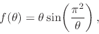$$f(\theta) = \theta\sin\!\left(\frac{\pi^{2}}{\theta}\right),$$ (50)

for $-\pi\leq\theta<0$ and $0<\theta\leq\pi$. It is well known that this function has an essential singularity at $\theta=0$ in the complex $\theta$ plane, which is an infinitely hard singularity. However, if defined by continuity at $\theta=0$ the function is continuous there, and therefore the singularity at $\theta=0$ is a soft one in the real sense of the term. The function is also continuous at all other points on the unit circle. We now observe that, despite having an infinitely hard complex singularity at $\theta=0$, this is a limited real function on a finite domain and therefore an integrable real function, which means that we may still construct an inner analytic function that corresponds to it. Presumably, this inner analytic function also has an essential singularity at the point $z=1$, which corresponds to $\theta=0$ on the unit circle. This fact would then prevent us from obtaining the value of the function at $\theta=0$ as the $\rho\to 1_{(-)}$ limit of the real part of that inner analytic function.

The mere fact that one can establish that there is a well defined inner analytic function for such a pathological real function is in itself rather unexpected and surprising. Furthermore, one can easily see that this is not the only example. One can also consider the related example, this time one in which the singularity is not soft in the real sense of the term,

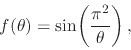$$f(\theta) = \sin\!\left(\frac{\pi^{2}}{\theta}\right),$$ (51)

which is still a limited real function on a finite domain and therefore an integrable real function, which again means that we may still construct an inner analytic function that corresponds to it. Many other variations of these examples can be constructed without too much difficulty.

Excluding all such exceptional cases, we may consider that the recovery of the real function $f(\theta)$ as the $\rho\to 1_{(-)}$ limit of the real part of the inner analytic function holds everywhere in the domain of definition of $f(\theta)$, that is, wherever it is well defined. In order to exclude all such exceptional cases, all we have to do is to exchange the condition that there be at most a finite number of hard singularities, in the real sense of the term, of the integrable real function $f(\theta)$, for the condition that there be at most a finite number of hard singularities with finite degrees of hardness, in the complex sense of the term, of the corresponding inner analytic function⁶ $w(z)$.

Once we have the inner analytic function that corresponds to a given integrable real function, we may consider the integral-differential chain to which it belongs. There are two particular cases that deserve mention here. One is that in which the inner analytic functions in the chain do not have any singularities at all on the unit circle, in which case the corresponding real functions are all analytic functions of $\theta$ in the real sense of the term. The other is that in which the inner analytic functions in the chain have only infinitely soft singularities on the unit circle, in which case the corresponding real functions are all infinitely differentiable functions of $\theta$, although they are not analytic. In this case one can go indefinitely along the chain in either direction without any change in the soft character of the singularities.

If, on the other hand, one does have borderline hard singularities or soft singularities with finite degrees of softness, then at some point along the chain there will be a transition to one or more hard singularities with strictly positive degrees of hardness, which do not necessarily correspond to integrable real functions. It can be shown that most of these singularities are instead associated to either singular distributions or non-integrable real functions. Their discussion will be postponed to the aforementioned forthcoming papers.