Next: Indexing in Momentum Space Up: Fourier Modes of a Previous: Fourier Modes of a
Just as we can represent the field in position space as a
![]() -dimensional real vector, so we would like to do the same in
momentum space. A real field
-dimensional real vector, so we would like to do the same in
momentum space. A real field ![]() on a
on a ![]() -lattice in
-lattice in ![]() dimensions
corresponds to
dimensions
corresponds to ![]() degrees of freedom, that is, to
degrees of freedom, that is, to ![]() independent real variables
independent real variables
![]() , one for each site of the
lattice, which is described by the integer coordinates
, one for each site of the
lattice, which is described by the integer coordinates ![]() . Since
Fourier transformation is simply a change of basis in the space of
functions on the lattice, from the position space representation
. Since
Fourier transformation is simply a change of basis in the space of
functions on the lattice, from the position space representation
![]() to the momentum-space representation
to the momentum-space representation
![]() , it follows that the Fourier components must also
include exactly
, it follows that the Fourier components must also
include exactly ![]() independent variables, one for each mode of the
lattice, which is described by the integer coordinates
independent variables, one for each mode of the
lattice, which is described by the integer coordinates
![]() . However, in its usual representation the Fourier transform of
a real scalar field is complex,
. However, in its usual representation the Fourier transform of
a real scalar field is complex,

and therefore seems to include twice as many real variables. This is not really so because not all such variables are independent, due to the identity
or, using the decomposition
![]() , the identities
, the identities
Besides, there are some modes for which the transform is real, such as
![]() , for which
, for which
![]() . So we see that counting
and keeping the truly independent variables is not so straightforward a
task.
. So we see that counting
and keeping the truly independent variables is not so straightforward a
task.
In order to keep just the ![]() independent variables, we must first
identify which modes are real and which modes are complex, and then adopt
some standard form of keeping the real and imaginary parts in a unique
way. A mode is real when
independent variables, we must first
identify which modes are real and which modes are complex, and then adopt
some standard form of keeping the real and imaginary parts in a unique
way. A mode is real when
![]() identically,
that is, for any field
identically,
that is, for any field
![]() , and is complex otherwise. For
example, it is clear that
, and is complex otherwise. For
example, it is clear that
![]() is real, as one can easily
verify by inspection of the definition of the transform. Since it is not
true in general that
is real, as one can easily
verify by inspection of the definition of the transform. Since it is not
true in general that
![]() , one can also
see from the definition that there are no purely imaginary modes. Hence
we have two classes of modes, purely real modes that contain a single
independent real variable each, and complex modes that contain two
mutually independent real variables each. These complex modes are related
in pairs by the identity above, so if we keep all of them we will be
double-counting the variables associated to them. For odd
, one can also
see from the definition that there are no purely imaginary modes. Hence
we have two classes of modes, purely real modes that contain a single
independent real variable each, and complex modes that contain two
mutually independent real variables each. These complex modes are related
in pairs by the identity above, so if we keep all of them we will be
double-counting the variables associated to them. For odd ![]() these
pairings can be illustrated by the diagram below, representing the
conjugate lattice in dimension
these
pairings can be illustrated by the diagram below, representing the
conjugate lattice in dimension ![]() ,
,
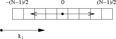
where every square represents a mode and one can see a vector ![]() as well as the negative of the same vector. In two dimensions we have the
corresponding diagram in figure 1. In these
diagrams one can see the limits of the range of the momentum coordinates
for odd
as well as the negative of the same vector. In two dimensions we have the
corresponding diagram in figure 1. In these
diagrams one can see the limits of the range of the momentum coordinates
for odd ![]() , which are
, which are ![]() and
and ![]() . The zero mode obviously
maps to itself. We see now that for odd
. The zero mode obviously
maps to itself. We see now that for odd ![]() there is a single real mode,
the zero mode, because all other modes map to a different mode inside the
conjugate lattice, by the inversion of the vector
there is a single real mode,
the zero mode, because all other modes map to a different mode inside the
conjugate lattice, by the inversion of the vector ![]() , due to the
fact that the extremes of the range are symmetrical. For even
, due to the
fact that the extremes of the range are symmetrical. For even ![]() the
situation is more complicated, in the case
the
situation is more complicated, in the case ![]() we have
we have
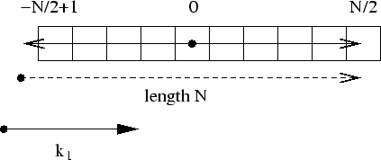
So we see that, because the extremes of the range of the variable are no
longer symmetrical, there is a mode, the mode ![]() , that maps to a
point outside the conjugate lattice, so that we must then add to the
inverted vector a period vector of length
, that maps to a
point outside the conjugate lattice, so that we must then add to the
inverted vector a period vector of length ![]() , as shown in the figure, in
order to bring it back into the conjugate lattice. As a consequence of
all this the mode
, as shown in the figure, in
order to bring it back into the conjugate lattice. As a consequence of
all this the mode ![]() also maps to itself, and is therefore a
real mode, as one may check by direct inspection of the definition of the
Fourier transform. In the case
also maps to itself, and is therefore a
real mode, as one may check by direct inspection of the definition of the
Fourier transform. In the case ![]() we have the diagram in
figure 2, were we see that in general many
modes will map to points outside the conjugate lattice, namely all those
modes that have at least one component equal to
we have the diagram in
figure 2, were we see that in general many
modes will map to points outside the conjugate lattice, namely all those
modes that have at least one component equal to ![]() , and in such cases
we must add a period vector of length
, and in such cases
we must add a period vector of length ![]() along one of the directions of
the lattice, as shown in the example depicted, with the period vector
along one of the directions of
the lattice, as shown in the example depicted, with the period vector
![]() . In some cases it may be necessary to add several period vectors
in different directions of the lattice, as in the case of the mode
. In some cases it may be necessary to add several period vectors
in different directions of the lattice, as in the case of the mode
![]() of this example, which needs two period vectors,
of this example, which needs two period vectors, ![]() and
and
![]() . However, not all such modes are real, because most times they
map to a different mode on the border of the lattice, as shown in the
example. In the case
. However, not all such modes are real, because most times they
map to a different mode on the border of the lattice, as shown in the
example. In the case ![]() we can see from the diagram that there will be
four real modes:
we can see from the diagram that there will be
four real modes: ![]() ,
, ![]() ,
, ![]() and
and ![]() .
.
In general we have ![]() real modes for even
real modes for even ![]() , and just one for odd
, and just one for odd
![]() . For odd
. For odd ![]() each complex mode is paired with the mode obtained by
the inversion of
each complex mode is paired with the mode obtained by
the inversion of ![]() , but for even
, but for even ![]() the pairings are not always
so simple, as there are modes paired within the surfaces with one
component equal to
the pairings are not always
so simple, as there are modes paired within the surfaces with one
component equal to ![]() . Nevertheless, all complex modes are dully
paired in this way. The idea for the classification of the
. Nevertheless, all complex modes are dully
paired in this way. The idea for the classification of the ![]() independent variables is that we leave the purely real modes alone and,
for each pair of conjugated complex modes, we keep only one real part and
one imaginary part. In order to have a conjugate lattice with one real
variable per site, just as have in position space for
independent variables is that we leave the purely real modes alone and,
for each pair of conjugated complex modes, we keep only one real part and
one imaginary part. In order to have a conjugate lattice with one real
variable per site, just as have in position space for
![]() ,
we must classify the modes in conjugate pairs and keep only the real part
of one member of the pair, and only the imaginary part of the other
member of the pair. As we do this we must also keep in mind that later on
we will index all the modes into a single
,
we must classify the modes in conjugate pairs and keep only the real part
of one member of the pair, and only the imaginary part of the other
member of the pair. As we do this we must also keep in mind that later on
we will index all the modes into a single ![]() -dimensional vector,
just as we do in position space.
-dimensional vector,
just as we do in position space.
On order to describe the scheme we adopt for this classification of
independent variables, we must discuss one dimension at a time. Starting
with ![]() , in this case we may simply keep the real parts of the modes
with positive components, and the imaginary parts of the modes with
negative components. In the simpler odd-
, in this case we may simply keep the real parts of the modes
with positive components, and the imaginary parts of the modes with
negative components. In the simpler odd-![]() case we represent this by the
diagram
case we represent this by the
diagram
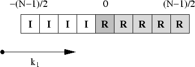
where the purely real modes are presented in a heavier shade, the complex modes of which we keep only the real parts in a lighter shade, and the complex modes of which we keep only the imaginary parts in white. The algorithm for implementing this is very simple,

In the even-![]() case, still for
case, still for ![]() , we have the diagram
, we have the diagram

and the algorithm is only slightly different,

For ![]() , in the odd-
, in the odd-![]() case, we adopt a scheme which is a
generalization of the previous one, and which is given by the diagram in
figure 3. We start by scanning the lattice
vertically by row, and define the situation on all horizontal rows that
do not contain a real mode. For each row that contains a real mode we
must examine the next coordinate. In this way we use the previous
case, we adopt a scheme which is a
generalization of the previous one, and which is given by the diagram in
figure 3. We start by scanning the lattice
vertically by row, and define the situation on all horizontal rows that
do not contain a real mode. For each row that contains a real mode we
must examine the next coordinate. In this way we use the previous ![]() scheme for the middle horizontal row of modes. The algorithm in this case
is a two-fold iteration of the algorithm for
scheme for the middle horizontal row of modes. The algorithm in this case
is a two-fold iteration of the algorithm for ![]() ,
,
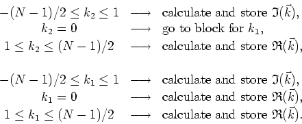
Note that we start by checking ![]() , not
, not ![]() , and only if it is
zero we go on to check
, and only if it is
zero we go on to check ![]() . In the even-
. In the even-![]() case, still for
case, still for ![]() , we
adopt a similar scheme, given by the diagram in
figure 4. Note that in this case the
, we
adopt a similar scheme, given by the diagram in
figure 4. Note that in this case the ![]() scheme is used for two horizontal rows, the middle one and the top
one. The algorithm in this case is once more a two-fold iteration of the
algorithm for
scheme is used for two horizontal rows, the middle one and the top
one. The algorithm in this case is once more a two-fold iteration of the
algorithm for ![]() ,
,
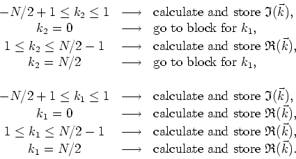
Note that in this case both the value ![]() and the value
and the value ![]() send us to test the next coordinate, so that there are two paths to get
from one block to the next block. Both the odd-
send us to test the next coordinate, so that there are two paths to get
from one block to the next block. Both the odd-![]() and the even-
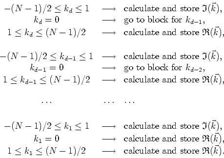
and the even-![]() algorithms can be easily generalized to arbitrary dimensions. Here is the
general algorithm for odd
algorithms can be easily generalized to arbitrary dimensions. Here is the
general algorithm for odd ![]() ,
,
Similarly, for even ![]() we have the general algorithm
we have the general algorithm
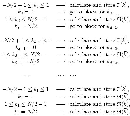
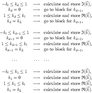
Note that, except for the changes in the minimum and maximum values of
each momentum coordinate, this algorithm includes the previous one, since
for odd ![]() a momentum coordinate will never have the value
a momentum coordinate will never have the value ![]() . Hence,
if we define
. Hence,
if we define ![]() to be
to be ![]() for odd
for odd ![]() and
and ![]() for even
for even ![]() , and define also
, and define also ![]() to be
to be
![]() where
the division indicated by the symbol
where
the division indicated by the symbol ![]() is integer division, with
truncation, so that
is integer division, with
truncation, so that ![]() is in fact
is in fact ![]() for odd
for odd ![]() and
and ![]() for even
for even ![]() , then we have the general algorithm, valid for both odd and
even
, then we have the general algorithm, valid for both odd and
even ![]() ,
,
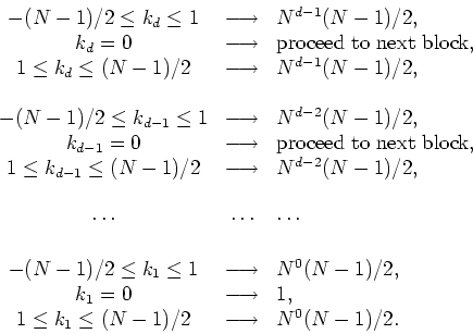
In the way of verification, one can count the number of modes which are
classified in each case. For odd ![]() we have, at each step of the
algorithm,
we have, at each step of the
algorithm,
Adding up all the contributions one gets
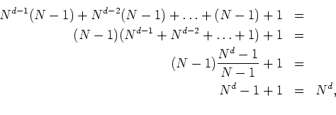
so that this case checks out. For even ![]() we have, at each step of the
algorithm,
we have, at each step of the
algorithm,
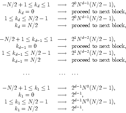
The factors of powers of ![]() that appear are due to the fact that there
are two ways to proceed from each block to the next one. Adding up all
the contributions one gets
that appear are due to the fact that there
are two ways to proceed from each block to the next one. Adding up all
the contributions one gets
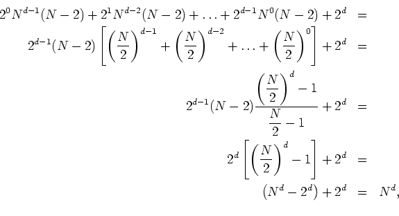
so that this case also checks out. Therefore, we have a completely well-defined algorithm that can be used to organize the independent variables, in any dimension. This algorithm should be used both when we calculate the Fourier components, in order to put them in their correct places in the conjugate lattice, and when one calculates an inverse transform or use the Fourier components in any other way, in order to get them from their correct places.