Next: Bibliography Up: Real Functions for Physics Previous: Conclusions
The fact that we discuss the properties of real functions only within the
interval ![]() is not a limitation from the physics point of view.
It is easy to show that all situations in physics application can be
reduced to this interval. Let us consider a physical variable
is not a limitation from the physics point of view.
It is easy to show that all situations in physics application can be
reduced to this interval. Let us consider a physical variable ![]() within
the closed interval
within
the closed interval ![]() , and let
, and let ![]() be a real function describing
some physical quantity within that interval. The size of the interval does
not matter. For example, if
be a real function describing
some physical quantity within that interval. The size of the interval does
not matter. For example, if ![]() is a measure of length, the interval could
be the size of a small resonant cavity or it could be the size of the
galaxy. In any case it is still a closed interval. The same is true if
is a measure of length, the interval could
be the size of a small resonant cavity or it could be the size of the
galaxy. In any case it is still a closed interval. The same is true if ![]() represents an energy, since it is always true that only limited amounts of
energy are available for any given experiment or realistic physical
situation. So long as
represents an energy, since it is always true that only limited amounts of
energy are available for any given experiment or realistic physical
situation. So long as ![]() , regardless of the magnitude or physical
nature of the dimensionfull physical variable
, regardless of the magnitude or physical
nature of the dimensionfull physical variable ![]() , we can rescale it to
fit within
, we can rescale it to
fit within ![]() . It is a simple question of making a change of
variables, by defining the new dimensionless variable
. It is a simple question of making a change of
variables, by defining the new dimensionless variable
so that
![]() . The inverse transformation is given by
. The inverse transformation is given by
The function ![]() can now be transformed into a function
can now be transformed into a function ![]() ,
,
where ![]() describes the same physics as
describes the same physics as ![]() . Let us now
consider the transformation of the first-order low-pass filter from one
system of variables to the other. Given a value of
. Let us now
consider the transformation of the first-order low-pass filter from one
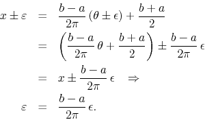
system of variables to the other. Given a value of ![]() , if we vary it
by
, if we vary it
by ![]() , we have a corresponding variation of
, we have a corresponding variation of ![]() , which we will
call
, which we will
call ![]() . It then follows that we have a relation between
. It then follows that we have a relation between
![]() and
and ![]() ,
,
The limit ![]() is now seen to be clearly equivalent to the
limit
is now seen to be clearly equivalent to the
limit
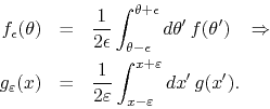
![]() , and the definition of the filtered function
, and the definition of the filtered function
![]() has a counterpart
has a counterpart
![]() ,
,
It follows that if ![]() is a combed function and we thus have that
is a combed function and we thus have that
then we also have that
so that ![]() is also a similarly combed function. We may thus conclude
that it suffices to consider and discuss only the set of combed functions
within
is also a similarly combed function. We may thus conclude
that it suffices to consider and discuss only the set of combed functions
within ![]() .
.